#FACEBOOK PREP
TOP RESOURCE: GAYLE SLIDES
"Interviewers rarely try to test knowledge of anything but the most basic Computer Science concepts. Instead, they are evaluating your ability to break down a tricky problem and to solve problems using what you do know."
HINT: BE HUMBLE, BE A GREAT TEAMMATE, BE GREAT ENGINEER, BE PASSIONATE, BE KNOWLEDGEABLE, BE CHALLENGEABLE
- SHOW YOU'RE SMART AND YOU CAN CODE
HINT: Memorize your CV: career, studies, accomplishment, hobbies, projects and past work.
I'M A MECHATRONICS ENGINEER WITH A PHD IN IT&C WITH A DISSERTATION FOCUSED ON AI AND MULTI-ROBOT CONTROL.
SINCE GRAD SCHOOL, I'VE BEEN DOING TECH FOR SOCIAL GOOD INCLUDING CIC.MX, A NON-PROFIT AWARDED BY ERIC
SCHMIDT'S NEW DIGITAL ERA GRANTS, WHICH WERE GIVEN TO THOSE PROMISING SOCIAL CAUSES WITH TECH BASIS. I'VE
DONE SEVERAL GEOREFERENCING PROJECTS CLOSE TO GOVERNMENT AND CIVIL SOCIETY ORGANIZATIONS, THOSE CONFORM MY
STRONGEST BASE IN SQL AND POSTGRESQL DATABASES. THEN I LEFT CIC.MX TO BUILD A STARTUP WITH A COUPLE OF
FRIENDS WHERE WE ARE BUILDING AN ALL-ACCESS API AND EASY TO READ DATA VISUALIZATIONS FROM OUR STATE-RUN
ELECTRICITY PROVIDER. WE'VE SUCCESSFULLY PULLED DATA FROM EVERY USER AND THE SYSTEM IS READY TO SCALE AS
ENGAGEMENT COMES. IN FACT THIS PROJECT MOTIVATED ME TO BUILD A MATERIAL-DESIGN BOILERPLATE, WHICH IS NOW
MY BIGGEST AND MOST PROMISING TECH ADVENTURE FOR EMPOWERING STARTUPS, ENTREPRENEURS AND NON-PROFITS DEV
TEAMS. THIS IS MOST OF MY TIME OUT OF WORK THAT IS STILL RELATED TO TECHNOLOGY, BESIDES, I'VE JUST
BECOME A DAD !
* DEEP DIVE INTO DISSERTATION AS A HARD|COOL PROJECT (HASHTABLE & JSON BASED TRANSFERS AND ALLOCATIONS)
* DEEP DIVE INTO MBOILERPLATE AS A HARD|COOL PROJECT (NOSQL, CLOUD BASED, SCALABLE, EXTENDIBLE, LOW-COST: SHOW
  HOW I LOVE TO BUILD STUFF FAST)
* THINK OF INCLUDING NIGHTS AND WEEKENDS: OPENCITYAPPS.MX, IPAB, EDUCTIVISM, EMULATED CDMA, NETWORK PALS...
1. GET INTERVIEW OUTFIT DRY CLEANED IF NECESSARY
2. REHEARSE STORIES FROM THE INTERVIEW PREP GRID
3. RE-READ 5 ALGORITH APPROACHES
4. CONTINUE TO PRACTICE UNTIL DAY OF INTERVIEW
5. REVIEW LIST OF TYPICAL MISTAKES
6. PRINT 10 COPIES OF MOST-UPDATED RESUME AND PUT THEM INTO FOLDER
7. AFTER: WRITE THANK YOU NOTE TO RECRUITER
DRESS CODE: KHAKIS, SLACKS OR NICE JEANS, POLO SHIRT OR DRESS SHIRT.
1. BE ENTREPRENEURIAL
2. ENHANCE A LOT MBOILERPLATE, SHOW HOW I LOVE TO BUILD STUFF FAST.
3. DEMONSTRATE "NINJA-SKILLS":
	3.1 HACK TOGETHER ELEGANT AND SCALABLE SOLUTIONS
	3.2 SHOW HOW YOU GET THINGS DONE
4. SHOW PASSION FOR AQUILA AND THE HARDWARE + SOFTWARE + HUMANITIES CROSSROADS
1. Tell Me About a Time When You Gave a Presentation to a Group of People Who Disagreed with You
2. Tell Me About the Biggest Mistake You Made on a Past Project
3. Tell Me About a Time When You Had to Deal with a Teammate Who Was Underperforming
4. Tell Me About a Time When You had to Make a Controversial Decision
5. Tell Me About a Time When You had to Use Emotional Intelligence to Lead
SKIR:
Scope the problem, Key clues and components, Issues, Repairs
DRIVE:
Lead the process and be open about issues, Do pseudocode before code
TEAMWORK:
Tweak, be open to feedback
PRACTICE:
Interview questions, coding on whiteboard, algorithms, design patterns
<span style="padding:5px; border-radius:4px; background-color:#7EB932; color:white;padding-left:20px; padding-right:40px"">KNOWLEDGE QUESTIONS
HINT: REVIEW CS FUNDAMENTALS AND KEY CONCEPTS

- Think on how-to SQL indexing, how-to design patterns, how-to webapp2
MEMORY (STACK VS HEAP)
**The Stack**: *global and local scope variables*
    What is the stack?
    It's a special region of your computer's memory that stores temporary
    variables created by each function (including the main() function). The
    stack is a "FILO" (first in, last out) data structure, that is managed and
    optimized by the CPU quite closely. Every time a function declares a new
    variable, it is "pushed" onto the stack. Then every time a function exits,
    all of the variables pushed onto the stack by that function, are freed (that
    is to say, they are deleted). Once a stack variable is freed, that region of
    memory becomes available for other stack variables.

    The advantage of using the stack to store variables, is that memory is
    managed for you. You don't have to allocate memory by hand, or free it once
    you don't need it any more. What's more, because the CPU organizes stack
    memory so efficiently, reading from and writing to stack variables is very
    fast.

    To summarize the stack:

		- the stack grows and shrinks as functions push and pop local variables
		- there is no need to manage the memory yourself, variables are
		  allocated and freed automatically
		- the stack has size limits
		- stack variables only exist while the function that created them, is
		  running

	Pros and cons:

		  very fast access
		  don't have to explicitly de-allocate variables
		  space is managed efficiently by CPU, memory will not become fragmented
		  local variables only
		  limit on stack size (OS-dependent)
		  variables cannot be resized
The Heap: global scope variables making use of pointers ( * )
	What is the heap?
	The heap is a region of your computer's memory that is not managed
	automatically for you, and is not as tightly managed by the CPU. It is a
	more free-floating region of memory (and is larger). To allocate memory on
	the heap, you must use malloc() or calloc(), which are built-in C
	functions. Once you have allocated memory on the heap, you are responsible
	for using free() to deallocate that memory once you don't need it any more.
	If you fail to do this, your program will have what is known as a memory
	leak. That is, memory on the heap will still be set aside (and won't be
	available to other processes). As we will see in the debugging sectio,
	there is a tool called valgrind that can help you detect memory leaks.

	Unlike the stack, the heap does not have size restrictions on variable size
	(apart from the obvious physical limitations of your computer). Heap memory
	is slightly slower to be read from and written to, because one has to use
	pointers to access memory on the heap.

	Unlike the stack, variables created on the heap are accessible by any
	function, anywhere in your program. Heap variables are essentially global
	in scope.

	Pros and cons:
		variables can be accessed globally
		no limit on memory size
		(relatively) slower access
		no guaranteed efficient use of space, memory may become fragmented over time as blocks of memory are allocated,
		then freed
		you must manage memory (you're in charge of allocating and freeing variables)
		variables can be resized using realloc()
Memory management in Python
	Memory management in Python involves a private heap containing all Python objects and data structures.
	The management of this private heap is ensured internally by the Python memory manager. The Python memory manager
	has different components which deal with various dynamic storage management aspects, like sharing, segmentation,
	preallocation or caching.

	It is important to understand that the management of the Python heap is performed by the interpreter itself and that
	the user has no control over it, even if she regularly manipulates object pointers to memory blocks inside that
	heap. The allocation of heap space for Python objects and other internal buffers is performed on demand by the
	Python memory manager through the Python/C API functions.

	locals() & gloabls() built-in functions output a dictionary of all in-memory variables
BIG-O


BIT MANIPULATION
	Implementation:
		 N = int('10000000000',2)
		 M = int('10011',2)
		 binary_m = bin(M)  #str in the form '0b10011'

	x << y
	Returns x with the bits shifted to the left by y places (and new bits on the right-hand-side are zeros).This is the same as multiplying x by 2**y.

	x >> y
	Returns x with the bits shifted to the right by y places. This is the same as dividing x by 2**y.

	x & y
	Does a "bitwise and". Each bit of the output is 1 if the corresponding bit of x AND of y is 1, otherwise it's 0.

	x | y
	Does a "bitwise or". Each bit of the output is 0 if the corresponding bit of x AND of y is 0, otherwise it's 1.

	~ x
	Returns the complement of x - the number you get by switching each 1 for a 0 and each 0 for a 1. This is the same as -x - 1.

	x ^ y
	Does a "bitwise exclusive or". Each bit of the output is the same as the corresponding bit in x if that bit in y is 0, and it's the complement of the bit in x if that bit in y is 1.
POWER OF 2
	2^7 = 128
	2^10 = ~1000 (1KB)
	2^20 = ~1000000 (1MB)
	2^30 = ~1000000000 (1GB)
	2^40 = ~1000000000000 (1TB)
RECURSION AND MEMOIZATION / DYNAMIC PROGRAMMING
**Typical use:**
    When there's a problem that can be built off of sub-problems.

    All recursive code can be implemented iteratively, although sometimes the code to do so is much more complex. Before diving into recursive code, ask yourself how hard it would be to implement it iteratively, and discuss the trade-offs with your interviewer.

    Hints for recursion:

    "Design an algorithm to compute the nth..."

    "Write code to list the first n"..."

    "Implement a method to compute all.. ."

    EXAMPLE:

    def hanoi(n, source, helper, target):
		print "hanoi( ", n, source, helper, target, " called"
		if n > 0:
    		# move tower of size n - 1 to helper:
    		hanoi(n - 1, source, target, helper)
    		# move disk from source peg to target peg
    		if source[0]:
        		disk = source[0].pop()
        		print "moving " + str(disk) + " from " + source[1] + " to " + target[1]
        		target[0].append(disk)
    		# move tower of size n-1 from helper to target
    		hanoi(n - 1, helper, source, target)

    source = ([4,3,2,1], "source")
	target = ([], "target")
	helper = ([], "helper")
	print source, helper, target
	hanoi(len(source[0]),source,helper,target)
	print source, helper, target
How-to Bottom-Up Recursion:
    1. Solve a simple case for single element.

    2. Extend previous solution for two elements.

    3. Then extend for three elements and so on. Typically fourth case is enough.

    The key here is to think about how you can build the solution for one case
    off of the previous case.
How-to Top-Down Recursion:
	1. Think how to divide proble for case N into subproblems.

	Be careful of overlap between the cases.
Slow recursive
	def fib(n):
		return n if n < 2 else fib(n-2) + fib(n-1)
Memoized
Memoisation is a technique used in computing to speed up programs. This is accomplished by memorizing the
	calculation results of processed input such as the results of function calls. If the same input or a function call
	with the same parameters is used, the previously stored results can be used again and unnecessary calculation are
	avoided. In many cases a simple array is used for storing the results, but lots of other structures can be used as
	well, such as associative arrays, called hashes in Perl or dictionaries in Python.

	def memoize(f):
		memo = {}
		def helper(x):
    		if x not in memo:
        		memo[x] = f(x)
    		return memo[x]
		return helper

	@memoize
	def fib(n):
		return n if n < 2 else fib(n-2) + fib(n-1)
MATH AND PROBABILITY
**Hints**
	1. Be careful with the difference in precision between floats and doubles.
	2. Don't assume that a value (such as the slope of a line) is an int unless you've been told so.
	3. Unless otherwise specified, do not assume that events are independent (or mutually exclusive). You should be careful, therefore, of blindly multiplying or adding probabilities.
Prime numbers
Every positive integer can be decomposed into a product of primes. Thus, in order for a number x to divide a number y (written x\y, or mod(y, x) = 0), all primes in x's prime factorization must be in y's prime factorization.

A list of primes a.k.a. The Sieve of Eratosthenes in Python:

	def sieveOfEratosthenes(n):
		"""return the list of the primes < n."""

		if n <= 2:
    		return []
		sieve = range(3, n, 2)
		top = len(sieve)
		for si in sieve:
    		if si:
        		bottom = (si*si - 3) // 2
        		if bottom >= top:
            		break
        		sieve[bottom::si] = [0] * -((bottom - top) // si)
		return [2] + [el for el in sieve if el]
Probability
A conditional 'intersection' of probabilities is calculated as the product of two or more probabilities (logical AND). Example given 1 to 10 (inclusive):

		P(A and B)=P(A)*P(B)
		P(x is even and x <= 5)
		= P(x is even given x <= 5) P(x <= 5) = (2/5) * (1/2)
		= 1/5


A conditional 'join' of probabilities is calculated as the sum of two or more probabilities (logical OR) minus the intersection. Example given 1 to 10 (inclusive):

		P(A or B)=P(A)+P(B)-P(A and B)
		P(x is even or x <=5)
		= P(x is even) + P(x <= 5) - P(x is even and x <= 5)
		= (1/2) + (1/2) - (1/5)
		= 4/5

Remember:
	 - independence means P(A and B)= P(A)*P(B).
	 - mutual exclusivity means P(A or B)=P(A)+P(B), since P(A and B)=0.
Permutations: (order does matter)
In mathematics, the notion of permutation relates to the act of arranging all the members of a set into some sequence or order, or if the set is already ordered, rearranging (reordering) its elements, a process called permuting.

	# (n)!/(n-r)! for n elements and r selections
	permutations('ABCD', 2)
	AB AC AD BA BC BD CA CB CD DA DB DC
Combinations: (order doesn't matter).
Combinations refer to the combination of n things taken k at a time without repetition. To refer to combinations in which repetition is allowed, the terms k-selection, k-multiset, or k-combination with repetition are often used.

	#(n)!/(r!(n-r)!) for n elements and r selections
	combinations('ABCD', 2)
	AB AC AD BC BD CD

	#(n+r-1)!/(r!(n-1)!) for n elements and r selections
	combinations_with_replacement('ABCD', 2)
	AA AB AC AD BB BC BD CC CD DD
OBJECT ORIENTED DESIGN (REAL-LIFE OBJECTS)
The implementation of classes and methods to sketch out technical problems or real-life objects.
How-to approach OOD
	STEP 1. Handle ambiguity

			Ask for clarifications, refer any possible assumption.
			Who's gonna use? How's gonna be used?
			Most detailed perspective should ask for who, what, where, when, how and why.

	STEP 2. Define the core objects

			Just after having a clear picture of what we're designing, lets list the core objects that conform our modeled solution.

	STEP 3. Analyze relationships

			Having more or less decided on our core objects, we now want to analyze the relationships between the objects.
			Which objects are members of which other objects?
			Do any objects inherit from any others?
			Are relationships many-to-many or one-to-many?

	STEP 4. Investigate actions

			At this point, you should have the basic outline of your object-oriented design. What remains is to consider the key actions that the objects will take and how they relate to each other. You may find that you have forgotten some objects, and you will need to update your design.

	STEP 5. Shall we use any Design Pattern ?
Python class pattern
	class Progression(object):
		""" <CLASS DOCUMENTATION> Iterator producing a generic progression.
		Default iterator produces the whole numbers 0, 1, 2, ...
		"""

		def __init__(self, start=0):
			"""<CONSTRUCTOR> Initialize current to the first value of the progression."""
			self._current = start

		def _advance(self):
			""" <INTERNAL METHOD WITH NO RETURN> Update self. current to a new value.
			This should be overridden by a subclass to customize progression.
			By convention, if current is set to None, this designates the
			end of a finite progression.
			"""
			self._current += 1

		def __next__(self):
			""" <INTERNAL METHOD WITH RETURN> Return the next element, or else raise StopIteration error."""
			if self._current is None: # our convention to end a progression
				raise StopIteration( )
			else:
				answer = self._current # record current value to return
				self._advance( ) # advance to prepare for next time
			return answer # return the answer

		def __iter__(self):
			""" <CONVENTIONAL METHOD> By convention, an iterator must return itself as an iterator."""
			return self

		def __str__(self):
			""" <CONVENTIONAL METHOD> By convention, reduce string representation of vector."""
			return "'" + self + "'"

		def print_progression(self, n):
			""" <OUTPUT METHOD> Print next n values of the progression."""
			print(' '.join(str(self.__next__()) for j in range(n)))

	class ArithmeticProgression(Progression): # inherits from Progression
		"""Iterator producing an arithmetic progression."""

		def __init__(self, increment=1, start=0):
			"""<INHERITANCE> Create a new arithmetic progression.
			increment the fixed constant to add to each term (default 1)
			start the first term of the progression (default 0)
			"""
			super(ArithmeticProgression, self).__init__(start) # initialize base class
			self._increment = increment

		def _advance(self): # override inherited version
			"""Update current value by adding the fixed increment."""
			self._current += self._increment


	def main():
		print( "Default progression:" )
		Progression().print_progression(10)
		Progression().print_progression(8)
		print( "Arithmetic progression with increment 5:" )
		ArithmeticProgression(5).print_progression(10)
		print( "Arithmetic progression with increment 5 and start 2:" )
		ArithmeticProgression(5, 2).print_progression(10)

	if __name__ == '__main__':
		main()
Singleton design pattern
	The Singleton pattern ensures that a class has only one instance and ensures access to the instance through the application without instantiating it again.

	# the python metaclass approach
	------

	class Singleton(type):
		def __call__(cls, *args, **kwargs):
    		try:
        		return cls.__instance
    		except AttributeError:
        		cls.__instance = super(Singleton, cls).__call__(*args, **kwargs)
        		return cls.__instance

	class MySingleton(object):
		__metaclass__ = Singleton
Factory design pattern
	The Factory pattern deals with the problem of creating objects without specifying the exact class of the object to be created. You give a parameter in order to know which class to instantiate.

	class A(object):
		def __init__(self):
		self.a = "Hello"

	class B(object):
		def __init__(self):
		self.a = " World"

	myfactory = {
		"greeting" : A,
		"subject" : B,
	}

	>>> print myfactory["greeting"]().a
	Hello
THREADS AND LOCKS
In computer science, a thread is used to run processes concurrently, meaning 2 or more sequences of programmed instructions could be running at the same time, sharing memory and the values of its variables at any given moment.
	Coordinating threads demands for additionals methods that ensure the concurrency won't affect the final desired result. Here come synchronization concepts such as: lock, rlock, condition, semaphore, events and queues.

		1. First of all, threading in python is through the threading.py standard module using the method .start(), i.e.:

			import threading
			class FetchUrls(threading.Thread):
				"""
					Thread checking URLs.
				"""

				def __init__(self, urls, output):
    				"""
    					Constructor.

    					@param urls list of urls to check
   						@param output file to write urls output
    				"""
    				threading.Thread.__init__(self)
    				self.urls = urls
    				self.output = output

				def run(self):
    				"""
    					Thread run method. Check URLs one by one.
    				"""
    				while self.urls:
        				url = self.urls.pop()
        				req = urllib2.Request(url)
        				try:
            				d = urllib2.urlopen(req)
        				except urllib2.URLError, e:
            				print 'URL %s failed: %s' % (url, e.reason)
        				self.output.write(d.read())
        				print 'write done by %s' % self.name
        				print 'URL %s fetched by %s' % (url, self.name)

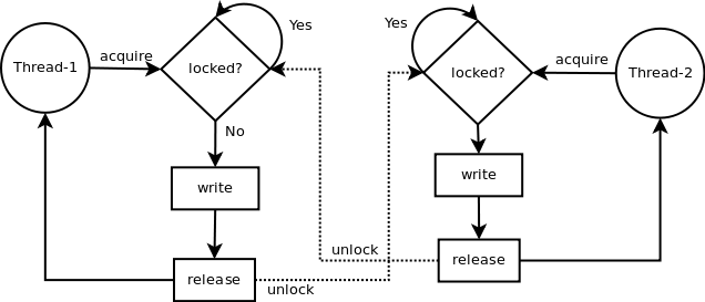
		2. Lock, used to enforce mutual exclusion and concurrency control to avoid a mess if doing same action like writing the same file, i.e.:

			class FetchUrls(threading.Thread):
				...

				def __init__(self, urls, output, lock):
   					...
    				self.lock = lock

				def run(self):
    				...
    				while self.urls:
        				...
        				self.lock.acquire()
        				print 'lock acquired by %s' % self.name
        				self.output.write(d.read())
        				print 'write done by %s' % self.name
        				print 'lock released by %s' % self.name
        				self.lock.release()
        				...
DATABASES
SQL Normalization: database that reduces data duplicity.
SQL Denormalization: databse that looks for highly scalable systems and faster queries (less joins).

NoSQL Leverages continual change in place, and speed of deployment.
DESIGN (recall How-to approach OOD)
SMALL DATABASE

		1. Handle ambiguity, find the level of detail or how general you should design.
		2. Define core objects, be aware that this information is typically the one that is redundant in denormalized systems.
		3. Analyze relationships, outline core objects and their relations including one-to-many, one-to-one, many-to-many.
		4. Investigate actions, define the most typical queries needed and re-structure if necessary.


LARGE DATABASE

		1. Follow the previous process but be redundant with most needed columns, denormalize your design.
		2. Don't be scared about duplicates, they're better than slow systems.
INDEXES
A database index is a data structure that improves the speed of data retrieval operations on a database table at the cost of additional writes and storage space to maintain the index data structure.

Indexes are special lookup tables that the database search engine can use to speed up data retrieval. Simply put, an index is a pointer to data in a table. An index in a database is very similar to an index in the back of a book.

Typical use implies trees or dictionaries with unique keys (B+Trees) that endup being bitmaps that identify data in a simpler representation.
SHARDING
A database shard is a horizontal partition of data in a database or search engine. Each individual partition is referred to as a shard or database shard. Each shard is held on a separate database server instance, to spread load.

Pros: reduced index size, which generally improves search performance.

Cons: heavier reliance on the interconnect between servers, increased latency when querying, issues of consistency, more complex failover and backups.
NoSQL
Focuses on large-volume and semi-structured data. Alleviates the problems that RDBMS imposes and makes it easy to work with large sparse data, but in turn takes away the power of transactional integrity and flexible indexing and querying.

MongoDB 4th most popular in the world, pretty much as Google's Datastore NDB, PostgreSQL and Cassandra. Leverage JSON or Binary-JSON (and even YAML and XML) structures instead of traditional relational databases (RDBMS). Useful in big data and real-time web apps and really attractive for programming modern web applications, which are subject to continual change in place, and speed of deployment is an important issue.

Google's Datastore NDB: Schemaless access, with SQL-like querying.

Classes:

	Column - JSONs with fixed properties: name, value and timestamp

	Document - most popular, flexible, designed to offer a richer experience with modern programming techniques

	Key-value - associative arrays or tuples

	Graph - semantic queries and graph structures.

	Multi-model - may use graph, relational and key-value models.
TASK QUEUES
Tasks queues are an efficient and powerful tool for background processing; they allow your application to define tasks, add them to a queue, and then use the queue to process them in aggregate.
Taskqueue lets applications to perform work outside of a user request, initiated by a user request. If an app needs to execute some background work, it can use the Taskqueues to organize that work into small, discrete units, called tasks. The app adds tasks to taskqueues to be executed later.
WEBAPP2 (Python WSGI)
A lightweight framework that allows you quickly build simple web applications for the Python 2.7 runtime. webapp2 is compatible with the WSGI standard for Python web applications.
WSGI is a specification for a standardized interface between Web servers and Python Web frameworks/applications. The goal is to provide a relatively simple yet comprehensive interface capable of supporting all interactions between a Web server and a Web framework.

Pros:
	- I no longer have to worry about making my application run in multiple Web servers: most servers, and all frameworks, are WSGI compliant.
	- WSGI is Python's Answer to Ruby On Rails
HINT: WHAT WHOULD YOU DO AT WORK ? BE REAL: GIVE AWAY THE WEBAPP, DATASTORE AND GOOGLE CLOUD SKILLS.

- Know Twitter, Facebook, Google, Amazon design architectures and why's.

FOLLOW-THROUGH
1. SCOPE THE PROBLEM
	1.1 IDENTIFY ALL POSSIBLE FEATURES AND FUNCTIONALITIES OF THE SYSTEM
2. STRUCTURE THE ARCHITECTURE
	2.1 USE WHITEBOARD TO DRAW ALL YOUR PIECES: FRONT-END, ROUTES, HANDLERS, AND MODELS
3. IDENTIFY KEY ISSUES
	3.1 IS YOUR APP WIRTE-HEAVY OR READ-HEAVY ? WHAT DOES THIS MEANS?
	3.2 HAVE YOU DETECTED BOTTLENECKS?
	3.3 SHOULD WE DISTRIBUTE THE DATABASE?
4. RESOLVE THE ISSUES
	4.1 THIS IS A GREAT MOMENT TO ASK FOR FEEDBACK
MODELING
Explains the best practices from twitter, amazon, google and facebook architectures.
.
Amazon
.
.
.
SCALABILITY & MEMORY LIMITS
**STEP BY STEP APPROACH**
	1. MAKE BELIEVE.
		Pretend that the data can all fit on one machine and there are no memory limitations.
		How would you solve the problem?
		This answer to this question will provide the general outline for your solution.
	2. GET REAL.
		 How much data can you fit on one machine, and what problems will occur when you split (shard) the data up?
		 Common problems include figuring out how to logically divide the data up,
		 and how one machine would identify where to look up a different piece of data.
	3. SOLVE PROBLEMS.
		Finally, think about how to solve the issues you identified in Step 2.
		Remember that the solution for each issue might be to actually remove the issue entirely,
		or it might be to simply mitigate the issue
HINTS FOR SHARDING
	* By Order of Appearance: advantage of never using more machines than are necessary. However, depending on the problem and our data set, our lookup table may be more complex and potentially very large.

	* By Hash Value: : (1) pick some sort of key relating to the data, (2) hash the key, (3) mod the hash value by the number of machines, and (4) store the data on the machine with that value. That is, the data is stored on machine #[mod(hash(key), N)].

	* By Actual Value: we may be able to reduce system latency by using information about what the data represents, for example geographic divisions.

	* Arbitrarily: Frequently, data just gets arbitrarily broken up and we implement a lookup table to identify which machine holds a piece of data. While this does necessitate a potentially large lookup table, it simplifies some aspects of system design and can enable us to do better load balancing.
SORTING AND SEARCHING
Understanding the common sorting and searching algorithms is incredibly valuable, as many of sorting and searching problems are tweaks of the well-known algorithms. A good approach is therefore to run through the different sorting algorithms and see if one applies particularly well.
SORTING
The most commonly used in interviews are:

* Mergesort
* Quicksort
* Bucket sort

Python sort and sorted methods use mergesort algorithms, thus being quasilinear in complexity.
SEARCHING
Master the following algorithms:

* Binary search
* Breadth first search (BFS)
* Depth first search (DFS)
* Binary tree traversal
UNIT TESTING
Unit testing is a software development process in which the smallest testable parts of an application, called units, are individually and independently scrutinized for proper operation.
It implies units associated with control data, usage procedures, and operating procedures, to be tested to determine whether they are fit for use.

In Python, there is the standard module unittest.py, i.e.:

	import unittest

	class TestUM(unittest.TestCase):

		def setUp(self):
    		pass

		def test_numbers_3_4(self):
    		self.assertEqual( 3*4, 12)

		def test_strings_a_3(self):
    		self.assertEqual( 'a'*3, 'aaa')

		def test_split(self):
  			s = 'hello world'
  			self.assertEqual(s.split(), ['hello', 'world'])
  			# check that s.split fails when the separator is not a string
  			with self.assertRaises(TypeError):
    			s.split(2)

	if __name__ == '__main__':
		unittest.main()
GOOGLE DATASTORE AND APPENGINE SCALABILITY
As previously referred, Google's Datastore is a managed, NoSQL, schemaless database for storing non-relational data. Cloud Datastore automatically scales as you need it and supports transactions as well as robust, SQL-like queries. It runs in the available instance of a given application.
App Engine applications are powered by any number of dynamic instances at a given time, depending on the volume of incoming requests. As requests for your application increase, so do the number of dynamic instances.

The App Engine scheduler decides whether to serve each new request with an existing instance (either one that is idle or accepts concurrent requests), put the request in a pending request queue, or start a new instance for that request. The decision takes into account the number of available instances, how quickly your application has been serving requests (its latency), and how long it takes to spin up a new instance.

Additionally, datastore scales by sharding rows onto separate tablet servers, and these rows are lexicographically ordered by key.
HINT: SHOW ANALYTICAL SKILLS, KEEP TRYING, COMMUNICATE YOUR THINKING, MAKE TRADEOFFS

- Master Big-O (Complexity), Trees and Graphs, MergeSort, BFS & DFS, Binary Search, Heaps, Recursion
- Python DS & Modules: List, Set, Dictionary, Itertools, Random, Collections, Heapq, Time; Functional Programming

FOLLOW-THROUGH
1. LISTEN
	1.1 PATTERN MATCHING: WHAT PROBLEM IS THIS SIMILAR TO ?
	1.2 GET CLUES
2. EXAMPLE
3. BRUTE FORCE
4. OPTIMIZE
	4.1 (B)OTTLENECKS
	4.2 (U)NNECESSARY WORK
	4.3 (D)UPLICATE WORK
5. EXPLAIN|WALKTHROUGH
6. IMPLEMENT|BEAUTIFY CODE: METHODS AND CLASSES
	6.1 CORRECT CODE
	6.2 EFFICIENT: BIG-O PERFORMANCE, METHODS RE-USE
	6.3 SIMPLE AND MODULAR
	6.4 READABLE
	6.5 MAINTAINABLE
	6.6 BALANCED USE OF DATA STRUCTURES
7. TEST
	7.1 ANALYZE: LOOKS WEIRD ? ERROR HOT SPOTS?
	7.2 TEST CASES: SMALL, EDGE, BIGGER
FIVE ALGORITHM APPROACHES
**1. EXAMPLIFY**
Write out specific examples until finding|deriving a rule of simplification or formula. Think of x equations (examples) and y variables.
2. PATTERN MATCHING
Think of familiarity and experience with past problems and modify solution in mind to the related problem. Most of the times a clue is found while carefully listening the problem description. Example: Clock angle.
3. SIMPLIFY & GENERALIZE
This is a multi-step approach useful when constraints are given. First we simplify a constraint such as the amount of data or memory, and solve for this simpler problem. Once we had it, we adapt the earlier solution for the more complex version. Example: Magazine words
4. BASE CASE AND BUILD
This is a useful approach when you find a clue for recursion. Try first to solve for n=1, then n=1 and n=2, and it's very possible for you to find a recursive approach when solved to n=4. Example: Permutations
5. DATA STRUCTURE BRAINSTORM
It's hacky and works. Use different data structures as examples and try to apply each one. You'll be surprised of how easy is to find the best data structure for your problem. Example: Median in growing array.
DATA STRUCTURES
* LIST
*Description:*

	The list type is a container that holds a number of other objects,
	in a given order. The list type implements the sequence protocol,
	and also allows you to add and remove objects from the sequence.

*Implementation:*

	l = [1,2,3]
	l = [1,'word',3]
	l[0] = 1

*Operations:*

	Operation     | Example      | Complexity       | Notes
	--------------+--------------+---------------+-------------------------------
	Index         | l[i]         | O(1)	         |
	Store         | l[i] = 0     | O(1)	         |
	Length        | len(l)       | O(1)	         |
	Append        | l.append(5)  | O(1)	         |
	Pop	          | l.pop()      | O(1)          | list as a stack (LIFO), same as l.pop(-1)
          		  | deque(l).popleft()           | list as a queue using collections.deque (FIFO)
	Clear         | l.clear()    | O(1)	         | similar to l = []

	Slice         | l[a:b]       | O(b-a)	     | l[1:5]:O(l)/l[:]:O(len(l)-0)=O(N)
	Extend        | l.extend(...)| O(len(...))   | depends only on len of extension
	Construction  | list(...)    | O(len(...))   | depends on length of argument

	check ==, !=  | l1 == l2     | O(N)          | O(len(string)) applies for strings
	Insert        | l[a:b] = ... | O(N)          |
          		  | l.insert(i,e)| O(N)	         | insert element e at zero-based index i
	Delete        | del l[i]     | O(N)	         |
	Remove        | l.remove(...)| O(N)	         |
	Containment   | x in/not in l| O(N)	         | searches list
	Copy          | l.copy()     | O(N)	         | Same as l[:] which is O(N)
	Pop           | l.pop(0)     | O(N)          |
	Index of      | l.index(e)   | O(N)          | return the zero-index index of element e
	Find          | l.find(e)    | O(N)          | return the zero-index index of element e or -1
	Index of      | l.rindex(e)  | O(N)          | return the zero-index index of element e from right to left
	Find          | l.rfind(e)   | O(N)          | return the zero-index index of element e or -1 from right to left
	Count         | l.count(e)   | O(N)          | return the occurrence of element e in l

	Extreme value | min(l)/max(l)| O(N)	         |
	Reverse	      | l.reverse()  | O(N)	         |
	Iteration     | for v in l:  | O(N)          |
            		l[::2]       | O(N)          | give all even indexes starting from 0
            		l[1::2]      | O(N)          | give all odd indexes starting from 1
            		l[::-1]      | O(N)          | reverses list

	Sort          | l.sort()     | O(N Log N)    | key/reverse change original l
          		  | sorted(l)    | O(N Log N)    | key/reverse doesn't change original l
	Multiply      | k*l          | O(k N)        | 5*l is O(N): len(l)*l is O(N**2)

*Typical use:*

    When you need a mixed collection of data all in one place.

    When the data needs to be ordered.

    When your data requires the ability to be changed or extended. Remember,
    lists are mutable.

    When you don't require data to be indexed by a custom value. Lists are
    numerically indexed and to retrieve an element, you must know its numeric
    position in the list.

    When you need a stack or a queue. Lists can be easily manipulated by
    appending/removing elements from the beginning/end of the list.

    When your data doesn't have to be unique. For that, you would use sets.

*Problem clues:*

	For regular list:

	For the stack implementation (append(), pop(), LIFO):

	For the deque implementation (append(), popleft(), FIFO):


* <span style="color: #FF4081">TUPLE</span>

	*Description:*

   		Tuples support all operations from lists that do not mutate the data structure
   		(and with the same complexity classes).

	*Implementation:*

		>>> l = (1,2,3)
		>>> l = (1,'word',3)
		>>> l[0]
		1
		>>> l[0] = 1
		TypeError: 'tuple' object does not support item assignment
-
SET
Description:
  A set is an unordered collection with no duplicate elements.
	Basic uses include membership testing and eliminating duplicate entries.
	Set objects also support mathematical operations like union, intersection,
	difference, and symmetric difference. Sets have many more operations that
	are O(1) compared with lists and tuples.

	Not needing to keep values in a specific order (which lists/tuples require)
	allows for faster operations.

	Frozen sets support all operations that do not mutate the data structure
	(and with the same complexity classes).
Implementation:
  s = set([1,2,3])


  EXAMPLES
  >>> A = {1, 2, 3, 3}
  >>> A
  set([1, 2, 3])
  >>> B = {3, 4, 5, 6, 7}
  >>> B
  set([3, 4, 5, 6, 7])
  >>> A | B     						# also works like A.union(B)
  set([1, 2, 3, 4, 5, 6, 7])
  >>> A & B     						# also works like A.intersection(B)
  set([3])
  >>> A - B     						# also works like A.difference(B)
  set([1, 2])
  >>> B - A     						# also works like B.difference(A)
  set([4, 5, 6, 7])
  >>> A ^ B     						# also works like A.symmetric_difference(B)
  set([1, 2, 4, 5, 6, 7])
  >>> (A ^ B) == ((A - B) | (B - A))
  True
  >>> A.issubset(B)					# test whether every element in s is in t
  False
  >>> A.issuperset(B)					# test whether every element in t is in s
  False
  >>> some_list = ['a', 'b', 'c', 'b', 'd', 'm', 'n', 'n']
  >>> duplicates = set([x for x in some_list if some_list.count(x) > 1])
  >>> print(duplicates)
  set(['b', 'n'])
Operations:
  Operation     | Example      | Complexity    | Notes
  --------------+--------------+---------------+-------------------------------
  Length        | len(s)       | O(1)	         |
  Add           | s.add(e)     | O(1)	         | adds element e as an insert(0,e)
  Containment   | x in/not in s| O(1)	         | compare to list/tuple - O(N)
  Remove        | s.remove(5)  | O(1)	         | compare to list/tuple - O(N)
  Discard       | s.discard(5) | O(1)	         |
  Pop           | s.pop()      | O(1)	         | compare to list - O(N), pops leftmost or FIFO
  Clear         | s.clear()    | O(1)	         | similar to s = set()
  Update        | s.update(t)  | O(len(s)+len(t))| return set s with elements added from t

  Construction  | set(...)     | len(...)      |
  check ==, !=  | s != t       | O(min(len(s),lent(t))
  <=/<          | s <= t       | O(len(s1))    | issubset
  >=/>          | s >= t       | O(len(s2))    | issuperset s <= t == t >= s
  Union         | s | t        | O(len(s)+len(t)) | concatenation
  Intersection  | s & t        | O(min(len(s),lent(t))  | coincidence elements, using &= returns set s keeping only elements also found in t
  Difference    | s - t        | O(len(t))     | s minus elements in t that are in s, using -= returns set s after removing elements found in t
  Symmetric Diff| s ^ t        | O(len(s))     | concatenation without coincidence elements, using ^= returns set s with elements from s or t but not both

  Iteration     | for v in s:  | O(N)          |
  Copy          | s.copy()     | O(N)	         |
Typical use:
  When you need a unique set of data: Sets check the unicity of elements
  based on hashes.
	When your data constantly changes: Sets, just like lists, are mutable.
	When you need a collection that can be manipulated mathematically: With
	sets it's easy to do operations like difference, union, intersection, etc.
	When you don't need to store nested lists, sets, or dictionaries in a data
	structure: Sets don't support unhashable types.
Problem clues:
. -
DICTIONARY
Description:
  Dictionaries are sometimes found in other languages as “associative
  memories” or “associative arrays”. Unlike sequences, which are indexed by a
  range of numbers, dictionaries are indexed by keys, which can be any
  immutable type; strings and numbers can always be keys. Most dict
  operations are O(1).

  It is best to think of a dictionary as an unordered set of key:value
  pairs, with the requirement that the keys are unique (within one
  dictionary). A pair of braces creates an empty dictionary: {}. Placing
  a comma-separated list of key:value pairs within the braces adds initial
  key:value pairs to the dictionary; this is also the way dictionaries are
  written on output.

  The main operations on a dictionary are storing a value with some key and
  extracting the value given the key. It is also possible to delete a
  key:value pair with del. If you store using a key that is already in use,
  the old value associated with that key is forgotten. It is an error to
  extract a value using a non-existent key.

  The keys() method of a dictionary object returns a list of all the keys
  used in the dictionary, in arbitrary order (if you want it sorted, just
  apply the sorted() function to it). To check whether a single key is in the
  dictionary, use the in keyword. The values() method returns a list of all
  values used.
Implementation:
  d = {'api_key': 'mwkMqTWFnK0LzJHyfkeBGoS2hr2KG7WhHqSGX0SbDJ4',
  		'container': 'CONTENTSHERE', 'channel': 'CHANNELHERE'}

  d = dict([('as',1),('king',10)])
Operations:
  Operation     | Example      | Complexity    | Notes
  --------------+--------------+---------------+-------------------------------
  Index         | d[k]         | O(1)	         | if k doesn't exists it throws KeyError
  Store         | d[k] = v     | O(1)	         |
  Length        | len(d)       | O(1)	         |
  Delete        | del d[k]     | O(1)	         |
  get/setdefault| d.method     | O(1)	         |
        		  | d.get(k)     | O(1)          | if k doesn't exists it throws None
  Pop           | d.pop(k)     | O(1)	         |
  Pop item      | d.popitem()  | O(1)	         | pops the first element as key,value tuple (FIFO)
  Clear         | d.clear()    | O(1)	         | similar to s = {} or = dict()
  Views         | d.keys()     | O(1)          | list of keys
        		  | d.values()   | O(1)          | list of values
        		  | d.items()    | O(1)	         | list of tuples as (key,value)

  Construction  | dict(...)    | len(...)      |

  Iteration     | for k in d:  | O(N)          | all forms: keys, values, items
  				for k,v in d.iteritems()     | for key, value pairs as k and v
Typical use:
  When you need a logical association between a key:value pair.
  When you need fast lookup for your data, based on a custom key.
  When your data is being constantly modified. Remember, dictionaries are
  mutable.
Problem clues:
.-
ORDEREDDICT
Implementation:
>>> from collections import OrderedDict >>> d = {'banana': 3, 'apple':4, 'pear': 1, 'orange': 2} >>> OrderedDict(sorted(d.items(), key=lambda t: t[0])) OrderedDict([('apple', 4), ('banana', 3), ('orange', 2), ('pear', 1)]) >>> OrderedDict(sorted(d.items(), key=lambda t: t[1])) OrderedDict([('pear', 1), ('orange', 2), ('banana', 3), ('apple', 4)]) -
DEFAULTDICT
Implementation:
>>> import collections >>> tree = lambda: collections.defaultdict(tree) >>> some_dict = tree() >>> some_dict['colours']['favourite'] = "yellow" #if this wasn't a defaultdict it'll have raised KeyError >>> import json >>> print(json.dumps(some_dict)) {"colours": {"favourite": "yellow"}} -
GRAPH
Description:
.Implementation:
  """ A Python Class
  A simple Python graph class, demonstrating the essential
  facts and functionalities of graphs.
  """


  class Graph(object):

      def __init__(self, graph_dict={}):
          """ initializes a graph object """
          self.__graph_dict = graph_dict

      def vertices(self):
          """ returns the vertices of a graph """
          return list(self.__graph_dict.keys())

      def edges(self):
          """ returns the edges of a graph """
          return self.__generate_edges()

      def add_vertex(self, vertex):
          """ If the vertex "vertex" is not in
              self.__graph_dict, a key "vertex" with an empty
              list as a value is added to the dictionary.
              Otherwise nothing has to be done.
          """
          if vertex not in self.__graph_dict:
              self.__graph_dict[vertex] = []

      def add_edge(self, edge):
          """ assumes that edge is of type set, tuple or list;
              between two vertices can be multiple edges!
          """
          edge = set(edge)
          (vertex1, vertex2) = tuple(edge)
          if vertex1 in self.__graph_dict:
              self.__graph_dict[vertex1].append(vertex2)
          else:
              self.__graph_dict[vertex1] = [vertex2]

      def __generate_edges(self):
          """ A static method generating the edges of the
              graph "graph". Edges are represented as sets
              with one (a loop back to the vertex) or two
              vertices
          """
          edges = []
          for vertex in self.__graph_dict:
              for neighbour in self.__graph_dict[vertex]:
                  if {neighbour, vertex} not in edges:
                      edges.append({vertex, neighbour})
          return edges

      def __str__(self):
          res = "vertices: "
          for k in self.__graph_dict:
              res += str(k) + " "
          res += "\nedges: "
          for edge in self.__generate_edges():
              res += str(edge) + " "
          return res

      def find_path(self, start_vertex, end_vertex, path=[]):
          """ find a path from start_vertex to end_vertex
              in graph """
          graph = self.__graph_dict
          path = path + [start_vertex]
          if start_vertex == end_vertex:
              return path
          if start_vertex not in graph:
              return None
          for vertex in graph[start_vertex]:
              if vertex not in path:
                  extended_path = self.find_path(vertex,
                                                 end_vertex,
                                                 path)
                  if extended_path:
                      return extended_path
          return None

      def find_all_paths(self, start_vertex, end_vertex, path=[]):
          """ find all paths from start_vertex to
              end_vertex in graph """
          graph = self.__graph_dict
          path = path + [start_vertex]
          if start_vertex == end_vertex:
              return [path]
          if start_vertex not in graph:
              return []
          paths = []
          for vertex in graph[start_vertex]:
              if vertex not in path:
                  extended_paths = self.find_all_paths(vertex,
                                                       end_vertex,
                                                       path)
                  for p in extended_paths:
                      paths.append(p)
          return paths

      def vertex_degree(self, vertex):
          """ The degree of a vertex is the number of edges connecting
              it, i.e. the number of adjacent vertices. Loops are counted
              double, i.e. every occurence of vertex in the list
              of adjacent vertices. """
          adj_vertices =  self.__graph_dict[vertex]
          degree = len(adj_vertices) + adj_vertices.count(vertex)
          return degree

      def find_isolated_vertices(self):
          """ returns a list of isolated vertices. """
          graph = self.__graph_dict
          isolated = []
          for vertex in graph:
              print(isolated, vertex)
              if not graph[vertex]:
                  isolated += [vertex]
          return isolated

      def delta(self):
          """ the minimum degree of the vertices """
          min = 100000000
          for vertex in self.__graph_dict:
              vertex_degree = self.vertex_degree(vertex)
              if vertex_degree < min:
                  min = vertex_degree
          return min

      def Delta(self):
          """ the maximum degree of the vertices """
          max = 0
          for vertex in self.__graph_dict:
              vertex_degree = self.vertex_degree(vertex)
              if vertex_degree > max:
                  max = vertex_degree
          return max

      def degree_sequence(self):
          """ calculates the degree sequence """
          seq = []
          for vertex in self.__graph_dict:
              seq.append(self.vertex_degree(vertex))
          seq.sort(reverse=True)
          return tuple(seq)

      def density(self):
          """ method to calculate the density of a graph """
          g = self.__graph_dict
          V = len(g.keys())
          E = len(self.edges())
          return 2.0 * E / (V *(V - 1))

  if __name__ == "__main__":

      g = { "a" : ["d"], "b" : ["c"], "c" : ["b", "c", "d", "e"], "d" : ["a", "c"], "e" : ["c"],"f" : []}

      graph = Graph(g)

      # or maybe
      >>> from collections import defaultdict
      >>> z = defaultdict()
  	>>> z["a"]=["d"]
  	>>> z["c"]=["b","c","d","e"]
  	>>> z["b"]=["c"]
  	>>> z["e"]=["c"]
  	>>> z["d"]=["a","c"]
  	>>> z["f"]=[]

  	graph = Graph(dict(z))
Operations:
  graph.vertices()
  graph.edges()
  graph.add_vertex("z")
  graph.add_edge({"a","z"})
  graph.density()
  graph.find_all_paths("a", "e")
Typical use:
.Problem clues:
. -
TREES
  Binary Tree vs. Binary Search Tree
  When given a binary tree question, many candidates assume that the interviewer means binary search tree. Be sure to ask whether or not the tree is a binary search tree. A binary search tree imposes the condition that, for all nodes, the left children are less than or equal to the current node, which is less than all the right nodes.

  Balanced vs. Unbalanced
  While many trees are balanced, not all are. Ask your interviewer for clarification on this issue. If the tree is unbalanced, you should describe your algorithm in terms of both the average and the worst case time. Note that there are multiple ways to balance a tree, and balancing a tree implies only that the depth of subtrees will not vary by more than a certain amount. It does not mean that the left and right subtrees are exactly the same size.

  Full and Complete
  Full and complete trees are trees in which all leaves are at the bottom of the tree, anD all non-leaf nodes have exactly two children. Note that full and complete trees are extremely rare, as a tree must have exactly 2n - 1 nodes to meet this condition

  Binary Tree Traversal
  Prior to your interview, you should be comfortable implementing in-order, post-order, and pre-order traversal. The most common of these, in-order traversal, works by visiting the left side, then the current node, then the right.
BINARY TREE
Description:
.Implementation:
  class BinaryTree():

  	def __init__(self,rootid):
  		self.left = None
  		self.right = None
  		self.rootid = rootid

  	def getLeftChild(self):
  		return self.left

  	def getRightChild(self):
  		return self.right

  	def setNodeValue(self,value):
  		self.rootid = value

  	def getNodeValue(self):
  		return self.rootid
Operations:
.Typical use:
.Problem clues:
.TRIE
Description:
A trie is a variant of an n-ary tree in which characters are stored at each node. Each path down the tree may represent a word.Implementation:
.Operations:
.Typical use:
.Problem clues:
.
-
args and kwargs
*args : additional arguments

>>> def test_var_args(f_arg, *argv):
....	print "first normal arg:", f_arg
....	for arg in argv:
....    	print "another arg through *argv :", arg

>>> test_var_args('yasoob','python','eggs','test')

>>> first normal arg: yasoob
>>> another arg through *argv : python
>>> another arg through *argv : eggs
>>> another arg through *argv : test

*kwargs : additional keyed arguments

>>> def greet_me(**kwargs):
....	if kwargs is not None:
....    	for key, value in kwargs.iteritems():
....        	print "%s == %s" %(key,value)

>>> greet_me(name="yasoob")
name == yasoob
Slicing
>>> a = [0, 1, 2, 3, 4, 5, 6, 7, 8, 9, 10]
>>> a[2:8]
[2, 3, 4, 5, 6, 7]

>>> a = [0, 1, 2, 3, 4, 5, 6, 7, 8, 9, 10]
>>> a[-4:-2]
[7, 8]

>>> a = [0, 1, 2, 3, 4, 5, 6, 7, 8, 9, 10]
>>> a[::2]
[0, 2, 4, 6, 8, 10]
>>> a[2:8:2]
[2, 4, 6]

>>> a = [0, 1, 2, 3, 4, 5, 6, 7, 8, 9, 10]
>>> a[::-1]
[10, 9, 8, 7, 6, 5, 4, 3, 2, 1, 0]
Enumerate
Similar to a dictionary, enumerate returns numeric-keyed value pairs as a list of tuples.

>>> seasons = ['Spring', 'Summer', 'Fall', 'Winter']
>>> list(enumerate(seasons))
[(0, 'Spring'), (1, 'Summer'), (2, 'Fall'), (3, 'Winter')]
Flattening
>>> a = [1, 2, [3, 4], [[5, 6], [7, 8]]]
>>> flatten = lambda x: [y for l in x for y in flatten(l)] if type(x) is list else [x]
>>> flatten(a)
[1, 2, 3, 4, 5, 6, 7, 8]
Zip
This function returns a list of tuples, where the i-th tuple contains the i-th element from each of the argument sequences or iterables. The returned list is truncated in length to the length of the shortest argument sequence.

>>> a = [1, 2, 3]
>>> b = ['a', 'b', 'c']
>>> z = zip(a, b)
>>> z
[(1, 'a'), (2, 'b'), (3, 'c')]
>>> zip(*z)
[(1, 2, 3), ('a', 'b', 'c')]

>>> x= [1,2,3]
>>> y=[4,5,6]
>>> [a+b for a,b in zip(x,y)]
[5, 7, 9]

#grouping
>>> a = [1, 2, 3, 4, 5, 6]
>>> group_adjacent = lambda a, k: zip(*([iter(a)] * k))
>>> group_adjacent(a, 3)
[(1, 2, 3), (4, 5, 6)]

#n grams
>>> from itertools import islice
>>> def n_grams(a, n):
...     z = (islice(a, i, None) for i in range(n))
...     return zip(*z)
...
>>> a = [1, 2, 3, 4, 5, 6]
>>> n_grams(a, 3)
[(1, 2, 3), (2, 3, 4), (3, 4, 5), (4, 5, 6)]

#inverting dict
>>> m = {'a': 1, 'b': 2, 'c': 3, 'd': 4}
>>> dict(zip(m.values(), m.keys()))
{1: 'a', 2: 'b', 3: 'c', 4: 'd'}
Filter
>>> def f(x): return x % 3 == 0 or x % 5 == 0
>>> filter(f, range(2, 25))
[3, 5, 6, 9, 10, 12, 15, 18, 20, 21, 24]
>>> number_list = range(-5, 5)
>>> less_than_zero = list(filter(lambda x: x < 0, number_list))
>>> less_than_zero
[-5, -4, -3, -2, -1]
Map
>>> def cube(x): return x*x*x
>>> map(cube, range(1, 11))
[1, 8, 27, 64, 125, 216, 343, 512, 729, 1000]
>>> items = [1, 2, 3, 4, 5]
>>> squared = map(lambda x: x**2, items)
[1, 4, 9, 16, 25]
# list comprehension approach
Reduce
>>> def add(x,y): return x+y
>>> reduce(add, range(1, 11))
55
List comprehension
Matrix of Zeros (WxL):
>>> zero_grid = [ [0] * W for j in range(L) ]

Filtering:
>>> [x for x in range(2,25) if x % 3 == 0 or x % 5 == 0]
[3, 5, 6, 9, 10, 12, 15, 18, 20, 21, 24]

Mapping:
>>> [x*x*x for x in range(1,11)]
[1, 8, 27, 64, 125, 216, 343, 512, 729, 1000]
Dictionary comprehension
>>> m = {x: 'A' + str(x) for x in range(10)}
>>> m
{0: 'A0', 1: 'A1', 2: 'A2', 3: 'A3', 4: 'A4', 5: 'A5', 6: 'A6', 7: 'A7', 8: 'A8', 9: 'A9'}
>>> {v: k for k, v in m.items()}
{'A1': 1, 'A0': 0, 'A3': 3, 'A2': 2, 'A5': 5, 'A4': 4, 'A7': 7, 'A6': 6, 'A9': 9, 'A8': 8}
Exceptions
Exception handling is an art which once you master grants you immense powers.

try:
	file = open('test.txt', 'rb')
except Exception as e:
	print('An error occurred: %s' % (format(e.args[-1])))
finally:
	print("This would be printed even if no exception occurs!")
Lambdas
Lambdas are one line functions. They are also known as anonymous functions in some other languages. You might want to use lambdas when you don’t want to use a function twice in a program. They are just like normal functions and even behave like them.

>>> add = lambda x, y: x + y
>>> print(add(3, 5))
8

>>> a = [(1, 2), (4, 1), (9, 10), (13, -3)]
>>> a.sort(key=lambda x: x[1])
>>> print(a)
# Output: [(13, -3), (4, 1), (1, 2), (9, 10)]
Built-ins
DIVMOD
>>> divmod(5,2)
(2, 1)
>>> 5 % 2
1

SORTING
>>> sorted([5, 2, 3, 1, 4])
[1, 2, 3, 4, 5]
>>> sorted([5, 2, 3, 1, 4], reverse=True)
[5, 4, 3, 2, 1]
>>> sorted("This is a test string from Andrew".split(), key=str.lower)
['a', 'Andrew', 'from', 'is', 'string', 'test', 'This']
>>> student_tuples = [
	('john', 'A', 15),
	('jane', 'B', 12),
	('dave', 'B', 10),
]
>>> sorted(student_tuples, key=lambda student: student[2])   # sort by age
[('dave', 'B', 10), ('jane', 'B', 12), ('john', 'A', 15)]
# same works for named objects:
>>> class Student:
    def __init__(self, name, grade, age):
        self.name = name
        self.grade = grade
        self.age = age
    def __repr__(self):
        return repr((self.name, self.grade, self.age))
>>> student_objects = [
	Student('john', 'A', 15),
	Student('jane', 'B', 12),
	Student('dave', 'B', 10),
]
>>> sorted(student_objects, key=lambda student: student.age)   # sort by age
[('dave', 'B', 10), ('jane', 'B', 12), ('john', 'A', 15)]

COMPLETE LIST
abs()	divmod()	input()	open()	staticmethod(
all()	enumerate()	int()	ord()	str()
any()	eval()	isinstance()	pow()	sum()
basestring()	execfile()	issubclass()	print()	super(
bin()	file()	iter()	property()	tuple()
bool()	filter()	len()	range()	type()
bytearray()	float()	list()	raw_input()	unichr()
callable()	format()	locals()	reduce()	unicode()
chr()	frozenset()	long()	reload()	vars()
classmethod()	getattr()	map()	repr()	xrange()
cmp()	globals()	max()	reversed()	zip()
compile()	hasattr()	memoryview()	round()	__import__()
complex()	hash()	min()	set()
delattr()	help()	next()	setattr()
dict()	hex()	object()	slice()
dir()	id()	oct()	sorted()
PYTHON USEFUL STANDARD IMPORTS
Itertools (python module)
itertools (https://docs.python.org/2.7/library/itertools.html)

		This module implements a number of iterator building blocks inspired by constructs from APL, Haskell, and SML. Each has been recast in a form suitable for Python.

	  	itertools.product('ABCD', repeat=2)	 					AA AB AC AD BA BB BC BD CA CB CC CD DA DB DC DD
		itertools.permutations('ABCD', 2)	 					AB AC AD BA BC BD CA CB CD DA DB DC
		itertools.combinations('ABCD', 2)	 					AB AC AD BC BD CD
		itertools.combinations_with_replacement('ABCD', 2)	 	AA AB AC AD BB BC BD CC CD DD
		itertools.product([0,1],repeat = 2)						00 01 10 11

EXAMPLE FOR COUNTING ALL PERMUTATIONS IN A GIVEN STRING
>>> import itertools
>>> z = []
>>> for i in itertools.permutations('abc',3): z.append(i)
>>> z
[('a', 'b', 'c'), ('a', 'c', 'b'), ('b', 'a', 'c'), ('b', 'c', 'a'), ('c', 'a', 'b'), ('c', 'b', 'a')]
>>> z_list = [a+b+c for a,b,c in z]
>>> z_list
['abc', 'acb', 'bac', 'bca', 'cab', 'cba']
>>> s = "abcabcabc"
>>> counter = 0
>>> for i in z_list: counter += s.count(i)
>>> counter
7
Random (python module)
random (https://docs.python.org/2.7/library/random.html)

	This module implements pseudo-random number generators for various distributions.
	For integers, uniform selection from a range. For sequences, uniform selection of a random element, a function
	to generate a random permutation of a list in-place, and a function for random sampling without replacement.

EXAMPLE

>>> random.random()        # Random float x, 0.0 <= x < 1.0
0.37444887175646646
>>> random.uniform(1, 10)  # Random float x, 1.0 <= x < 10.0
1.1800146073117523
>>> random.randint(1, 10)  # Integer from 1 to 10, endpoints included
7
>>> random.randrange(0, 101, 2)  # Even integer from 0 to 100
26
>>> random.choice('abcdefghij')  # Choose a random element
'c'
>>> items = [1, 2, 3, 4, 5, 6, 7]
>>> random.shuffle(items)
>>> items
[7, 3, 2, 5, 6, 4, 1]
>>> random.sample([1, 2, 3, 4, 5],  3)  # Choose 3 elements
[4, 1, 5]
Collections (python module)
collections (https://docs.python.org/2.7/library/collections.html)

		This module implements specialized container datatypes providing alternatives to Python’s general purpose built-in containers, dict, list, set, and tuple.

		collections.Counter			dict subclass for counting hashable objects
		collections.deque			list-like container with fast appends and pops on either end
		collections.OrderedDict		dict subclass that remembers the order entries were added

		collections.defaultdict		dict subclass useful for trees (calls a factory function)

EXAMPLE COUNTER
>>> Counter('abracadabra').most_common(3)
[('a', 5), ('r', 2), ('b', 2)]
>>> import re
>>> words = re.findall(r'\w+', open('hamlet.txt').read().lower())
>>> Counter(words).most_common(4)
[('the', 1143), ('and', 966), ('to', 762), ('of', 669)]

EXAMPLE DEQUE
>>> queue = deque(["Eric", "John", "Michael"])
>>> queue.append("Terry")           # Terry arrives
>>> queue.append("Graham")          # Graham arrives
>>> queue.popleft()                 # The first to arrive now leaves
'Eric'
>>> queue.popleft()                 # The second to arrive now leaves
'John'
>>> queue                           # Remaining queue in order of arrival
deque(['Michael', 'Terry', 'Graham'])
>>> Q = deque([5, 2, 1, 3])
>>> Q.rotate(3)
deque([2, 1, 3, 5])
>>> def moving_average(iterable, n=3):
		# moving_average([40, 30, 50, 46, 39, 44]) --> 40.0 42.0 45.0 43.0
		# http://en.wikipedia.org/wiki/Moving_average
		it = iter(iterable)
		d = deque(itertools.islice(it, n-1))
		d.appendleft(0)
		s = sum(d)
		for elem in it:
    		s += elem - d.popleft()
    		d.append(elem)
    		yield s / float(n)

EXAMPLE ORDEREDDICT
>>> d = {'banana': 3, 'apple':4, 'pear': 1, 'orange': 2}
>>> OrderedDict(sorted(d.items(), key=lambda t: t[0]))
OrderedDict([('apple', 4), ('banana', 3), ('orange', 2), ('pear', 1)])
>>> OrderedDict(sorted(d.items(), key=lambda t: t[1]))
OrderedDict([('pear', 1), ('orange', 2), ('banana', 3), ('apple', 4)])

EXAMPLE DEFAULTDICT
>>> import collections
>>> tree = lambda: collections.defaultdict(tree)
>>> some_dict = tree()
>>> some_dict['colours']['favourite'] = "yellow"    #if this wasn't a defaultdict it'll have raised KeyError
>>> import json
>>> print(json.dumps(some_dict))
{"colours": {"favourite": "yellow"}}
Heapq (python module)
heapq (https://docs.python.org/2.7/library/heapq.html)

	This module provides an implementation of the heap queue algorithm, also known as the priority queue algorithm.
	Heaps are binary trees for which every parent node has a value less than or equal to any of its children. This
	implementation uses arrays for which heap[k] <= heap[2*k+1] and heap[k] <= heap[2*k+2] for all k, counting
	elements from zero. For the sake of comparison, non-existing elements are considered to be infinite. The
	interesting property of a heap is that its smallest element is always the root, heap[0].

EXAMPLE

>>> from heapq import heappush, heappop
>>> def heapsort(iterable):
...     h = []
...     for value in iterable:
...         heappush(h, value)
...     return [heappop(h) for i in range(len(h)]
>>> heapsort([1, 3, 5, 7, 9, 2, 4, 6, 8, 0])
[0, 1, 2, 3, 4, 5, 6, 7, 8, 9]
Time (python module)
time (https://docs.python.org/2.7/library/time.html)

	This module is useful for testing complexity and computational cost in terms of time.

EXAMPLE

>>> from time import time
>>> def InsertionSort(A):
...		start_time = time() # record the starting time
...		for j in range(1, len(A)):
...			key = A[j]
...			i = j - 1
...			while (i >=0) and (A[i] > key):
...				A[i+1] = A[i]
...				i = i - 1
...			A[i+1] = key
...		end_time = time() # record the ending time
...		elapsed = end_time - start_time
...		print "Elapsed time (ms): %s" % (elapsed)
...		return A
Math (python module)
math (https://docs.python.org/2/library/math.html)

	This module is always available. It provides access to the mathematical functions defined by the C standard.

EXAMPLE

>>> import math
>>> math.pi
3.141592653589793
>>> math.sin(math.pi/2)
1.0
>>> math.log(4,2)
2.0
>>> math.factorial(4)
24
re (python module)
re (https://docs.python.org/2/howto/regex.html)

	This module provides Perl-style regular expression patterns.

>>> import re
>>> words = re.findall(r'\w+', open('hamlet.txt').read().lower())

>>> p = re.compile('\d+')
>>> p.findall('12 drummers drumming, 11 pipers piping, 10 lords a-leaping')
['12', '11', '10']

>>> p = re.compile(r'(\b\w+)\s+\1')
>>> p.search('Paris in the the spring').group()
'the the'

>>> p = re.compile( '(blue|white|red)')
>>> p.sub( 'colour', 'blue socks and red shoes')
'colour socks and colour shoes'
ALGORITHMS
**SORT**
Is worth to refer that python exercises of sorting algorithms provide the following leading results:
	1) Numpy
    2) Native
    3) Quicksort list comprehension
    4) Mergesort
-
MERGE-SORT
Merge sort is a recursive algorithm that continually splits a list in half. If the list is empty or has one item, it is sorted by definition (the base case). If the list has more than one item, we split the list and recursively invoke a merge sort on both halves. def mergeSort(alist): print("Splitting ",alist) if len(alist)>1: mid = len(alist)//2 lefthalf = alist[:mid] righthalf = alist[mid:] mergeSort(lefthalf) mergeSort(righthalf) i=0 j=0 k=0 while i < len(lefthalf) and j < len(righthalf): if lefthalf[i] < righthalf[j]: alist[k]=lefthalf[i] i=i+1 else: alist[k]=righthalf[j] j=j+1 k=k+1 while i < len(lefthalf): alist[k]=lefthalf[i] i=i+1 k=k+1 while j < len(righthalf): alist[k]=righthalf[j] j=j+1 k=k+1 print("Merging ",alist) alist = [54,26,93,17,77,31,44,55,20] mergeSort(alist) print(alist) -
QUICK-SORT
  Quick sort is a recursive algorithm that continually splits a list according to a pivotValue. If the list is empty or has one item, it is sorted by definition (the base case). If the list has more than one item, we split the list with all values below pivot in one side and all values above pivot on another side, and recursively invoke a quick sort on both side.

  Python methods work faster in Big-O, but an implementation of quick sort can be:

  def quickSort(list):
  	"""Quicksort using list comprehensions"""
  	if list == []:
  		return []
  	else:
  		pivot = list[0]
  		lesser = quickSort([x for x in list[1:] if x < pivot])
  		greater = quickSort([x for x in list[1:] if x >= pivot])
  		return lesser + [pivot] + greater

  alist = [54,26,93,17,77,31,44,55,20]
  alist = quickSort(alist)
  print(alist)
SEARCH
-
GRAPH SEARCH
Breadth first and depth first are useful graph traversal and searching algorithms. DFS is typically the easiest if we want to visit every node in the graph, or at least visit every node until we find whatever we're looking for. However, if we have a very large tree and want to be prepared to quit when we get too far from the original node, DFS can be problematic; we might search thousands of ancestors of the node, but never even search all of the node's children. In these cases, BFS is typically preferred This is an excellent representation in python. Given the graph implementation in section Data Structures: def find_path(self, start_vertex, end_vertex, path=[]): """ find a path from start_vertex to end_vertex in graph """ graph = self.__graph_dict path = path + [start_vertex] if start_vertex == end_vertex: return path if start_vertex not in graph: return None for vertex in graph[start_vertex]: if vertex not in path: extended_path = self.find_path(vertex, end_vertex, path) if extended_path: return extended_path return None def find_all_paths(self, start_vertex, end_vertex, path=[]): """ find all paths from start_vertex to end_vertex in graph """ graph = self.__graph_dict path = path + [start_vertex] if start_vertex == end_vertex: return [path] if start_vertex not in graph: return [] paths = [] for vertex in graph[start_vertex]: if vertex not in path: extended_paths = self.find_all_paths(vertex, end_vertex, path) for p in extended_paths: paths.append(p) return paths -
BINARY SEARCH
  After sorting an array, binary search is a useful algorithm based on divide and conquer.

  		def binary_search(S, target):
  			"""Return True if target found, else False."""
  			start = 0
  			stop = len(S)
  			if start >= stop: # zero elements in slice
  				return False
  			else: # two or more elements in slice
  				mid = (start + stop) // 2
  			if target == S[mid]:
  				return True
  			elif target > S[mid]:
  				return binary_search(S[mid+1:], target)
  			else:
  				return binary_search(S[:mid-1], target)
HINT: HANDLE THE POST-INTERVIEW STRESS
- Think of deadlines and extensions if necessary
- Handle with care if you think to decline, keep a line of communication open
AND YOUR REAL SALARY IS...
+ OFFER SALARY
This is your periodical income.
-
SIGNING BONUS, RELOCATION AND ONE-TIME PERKS
When comparing offers, it's wise to amortize this cash over three years (or however long you expect to stay).
-
COST OF LIVING DIFFERENCE
Silicon Valley, for example, is about 20 to 30% more expensive than Seattle.
-
ANNUAL BONUS
This ranges from anywhere from 3% to 30%.
-
STOCK OPTIONS AND GRANTS
Equity compensation can form another big part. Amortize this cash over three years and lump that value into salary.
-
PROMOTION PLAN
This is not money in your pocket, but it can or can't be in your near future in the company.
-
HAPPINESS FACTOR
Think of the product, the culture, working hours, and if possible meet your Manager and Teammates.