The price predictor algorithm predicts two attributes. First one is the DTS(estimated Days To Sell) and the second one is the price of the given Sneaker. The algorithm does so by taking Brand Name, Size, and Condition of the shoe. The algorithm predicts both of the attributes using random forest regressor. The dataset used to train the algorithm was obtained from Swag Kicks sold sneakers data. The SK_ShoesPricePredictorv2 is a part of the price suggester algorithm for the sneakers.
RandomForestRegressor-based price predictor model is based on three pillars:
- Dataset - made from the historical data of the sneakers sold on SwagKicks
- Python Code - Where the dataset is processed and run through the Random Forest Regressor Algorithm due to which we are able to predict the price.
- API - the required fields are sent as attributes to our API the response of which is shown on the website as the suggested price.
The initial dataset consisted of Product Title, Size, Date Sold At, Product Created Date, Condition, Barcode, Variant SKU, and Product Price.
This was arguably the hardest part of the whole process. First and foremost what I had to do is to restore as much data as possible, as the in the initial data there were alot of products where the Size and Condition attributes were missing. To do that I had to gather data from other sources such as uploading data, and the data on thriftops so that we don't miss those tasty rows which are going to help us getting more and more accurate results.
With getting the missing data out of the way next task was to determine the DTS of each article - which was as easy as subtracting two values in excel. (It was actually just that)
At this time the headers of our sheet look something like Product Title, Size, DTS, Condition, SKU, and Product Price. (Merged barcode and SKU)
Next I want to get rid of SKU. So I will be doing a last check on SKU by applying a sort filter and checking if there is something other than the Sneakers in the dataset and sure as expected I did found some data which wasn't of Sneakers. With this step we are done with the SKU column too.
Now we are on the last part of the Wrangling step which is to extract the brands out of the product title, and let me tell you this isn't fun at all. So lets make a new column and name it "Brands" so that we can start filling it up. So the easiest way of going by this IMO is to first populate the rows where the brand name is there in the title without the typos. Luckily I have been through this earlier so I already have a list of the major brand we have in good quantity. So, with the magic of excel filters I got onto that.
Once I am done with that now its time to find the ones with typos in them. One of the easiest way is to use the sort - as most of the titles have brand name at the begining. This way it is much easier to identify the brand names with typos so I kept on filling the "Brand" column with the respective brands. In the process I saw that there are many brands which didn't had much volume in the old dataset so I had to label them too. After that all the smaller brands went under the umbrella of "Others".
Last thing I did which is the major difference between v1 and v2 is the "Premium" column. So, earlier in v1 what I did is labelled any sneaker sold over Rs. 5.5k as BrandName+" Premium" e.g a Nike shoe sold for Rs.6000 was labeled as Nike Premium in the brand column. While working on v2 I realized that this gives us a limitiation(discussed later in the report).
Finally after deleting the title column we are left with Brand, Premium, Size, Condition, Product Price, and DTS which is our final dataset.
So according to me the biggest difference in the v1 and v2 is the addition of the "Premium" column. So, as discussed earlier that in v1 what I did is labelled any sneaker sold over Rs. 5.5k as BrandName+" Premium" e.g a Nike shoe sold for Rs.6000 was labeled as Nike Premium in the brand column. While working on v2 I realized that this gives us a limitiation. In v1 lets say there is a brand X which have like 256 rows and all of the rows are of non-premium. Lets assume that in v1 we trained the dataset and now when there is a shoe of brand X which lies in premium category the algorithm will fail to provide its data. On the other hand if we have a seperate column for premium category and we keep cohesion between the brand name and premium tag we can resolve the issue of getting premium predictions on the untrained brands. Other than this issue the data for each brand gets increases as in v1 Nike and Nike Premium were treated as two different entities. Now in v2 - Nike and Nike (1 in Premium) are trated as a single entity and Premium on the other hand has all the data to work and train.
Datasets may or may not have some outliers. An outlier is an observation that lies an abnormal distance from other values in a random sample from a population. So in out case all the sneakers sold under Rs. 500 and the sneakers sold above Rs. 25k are outliers in terms of price. For DTS I decided to delete the sneakers where DTS > 600.
The algorithm is trained in Python language. In the initial parts of the code some basic wrangling is performed.
After that depending on the algorithm(DTS, or Price) the dataset is seperated into X and Y arrays. Using Scikit library the data is randomly splitted for testing and training. In our case the split is 30-70, that is 30% for testing and 70% of the dataset to be used for training the algoritm .
As the ML algorithms don't understand text One Hot Encoder is used on Brand and Condition to make it readable for the algorithm. This step is stored in the pipeline as SK Pipeline library was used in training the algorithm.
Next the algorithm is trained using the RandomForestRegressor and then a pickle is created for each (DTS and Price algorithm).
Whatever we discussed so far about the code was the part where we trained the algorithm. Now the next challange is to send the inputs into the algorithm and getting the desired outputs from it.
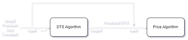
In v2 there are two algorithms working in sequence. The first algorithm takes Brand, Premium, Size, and Condition as inputs and return the predected DTS for that shoe. After that the second algorithm gets triggered which automatically takes all the inputs from the first algorithm as well as the output of the first algorithm as the inputs. Finally the second algorithm returns the predicted price of the sneaker. The API's output is predicted DTS and Price (comma sperated)
Future Works:
Determine the condition on its own. Predict the price on the bases of title rather than the brand name.