PySourceviz

English | 简体中文

PySourceviz turns MNE-Python cortical source estimates into consistent, publication-friendly surface figures with a selectable BrainSpace or Nilearn renderer. It keeps source-estimate semantics in MNE, uses FreeSurfer anatomy for the mesh and medial wall, and renders four comparable views with one whole-brain activation colorbar.

The v0.1 visual defaults are an inflated cortical surface, white background, soft white-to-light-gray sulcal shading, a transparent low-value overlay, and this anatomical order:

LH lateral | LH medial | RH medial | RH lateral

For source-localization overview figures, PySourceviz recommends the inflated surface used by default in mne.SourceEstimate.plot. Inflation exposes activation that would be hidden inside sulci and avoids visually equating detailed fold boundaries with the spatial resolution of the inverse solution. It changes only display coordinates: source vertices, activation values, timing, interpolation, thresholds, and color limits remain unchanged. pial and white remain available when their anatomy is the intended subject of the figure.

Result gallery

PySourceviz · MNE audvis dSPM · inflated surface · 110 ms actual sample

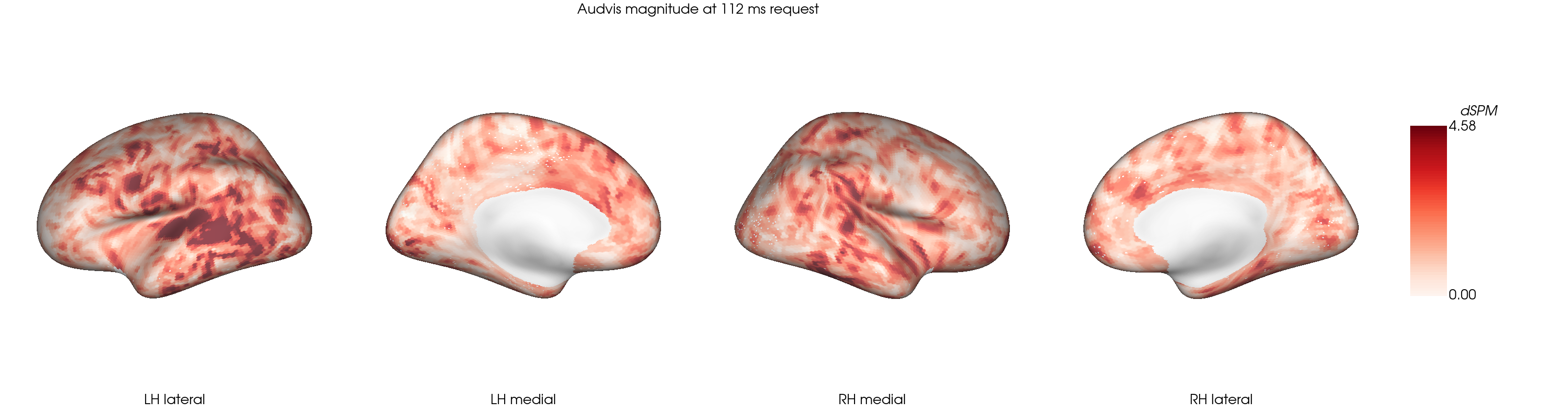
The requested time above is 112 ms. The STC is sampled every 10 ms, so PySourceviz selects 110 ms and records that actual sample in the returned metadata.

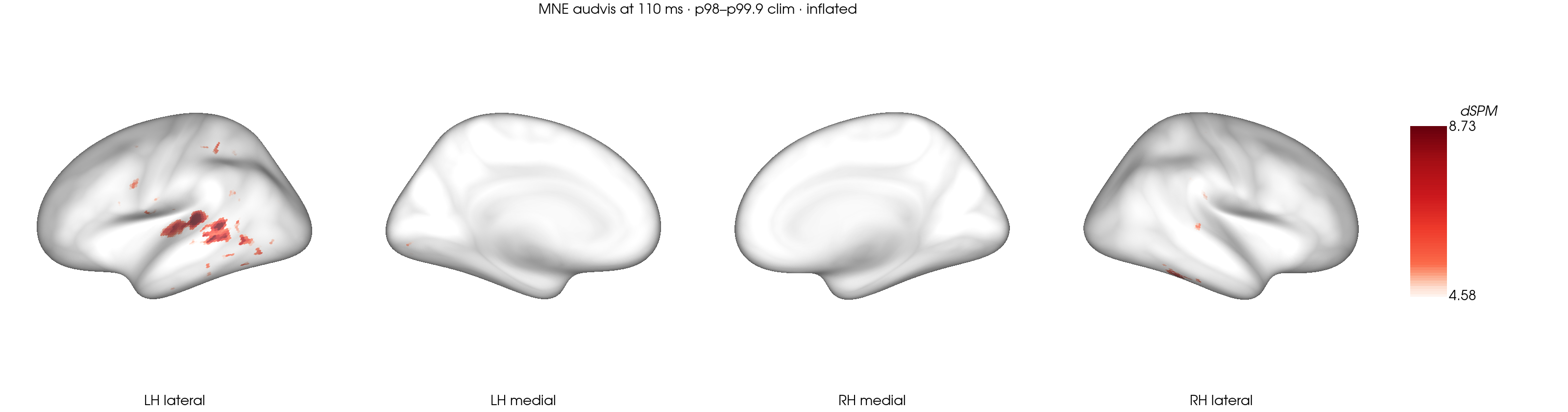
PySourceviz · BrainSpace backend · inflated surface · p98-p99.9 color controls

PySourceviz · Nilearn backend · inflated surface · the same activation and limits

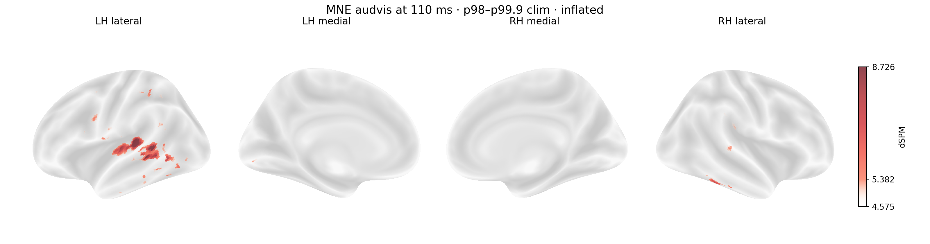
Both images above are produced by built-in PySourceviz backends. They use the same STC and time sample. They also use the same inflated geometry, expanded vertex values, medial-wall mask, FreeSurfer sulc background, colormap, and color limits; only the final renderer changes. The white-gray texture is therefore retained on the inflated coordinates rather than being tied to pial geometry.

PySourceviz · BrainSpace · pial surface · optional anatomical view

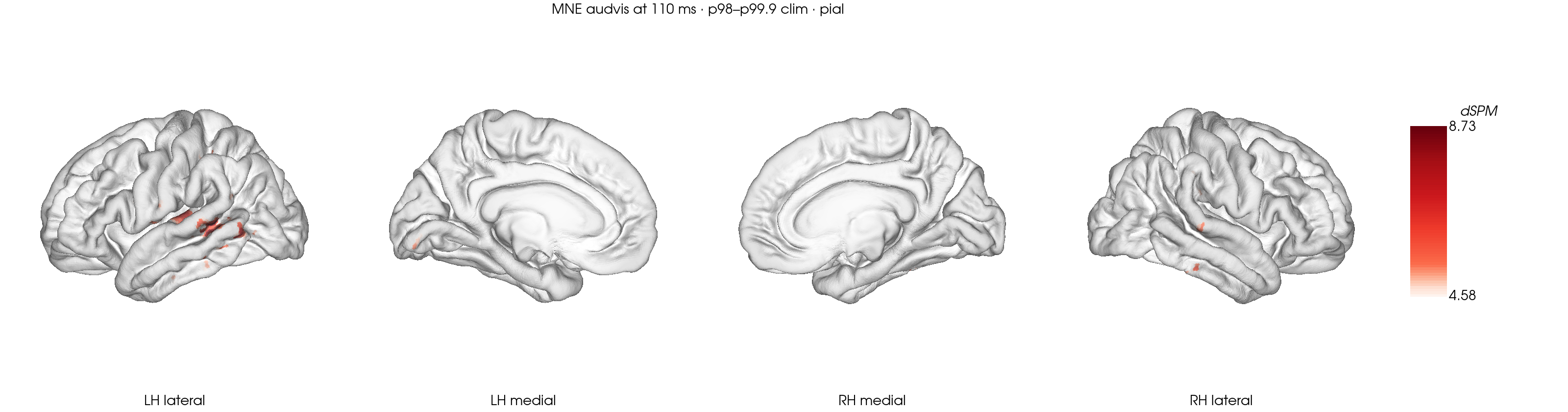
PySourceviz · Nilearn · pial surface · optional anatomical view

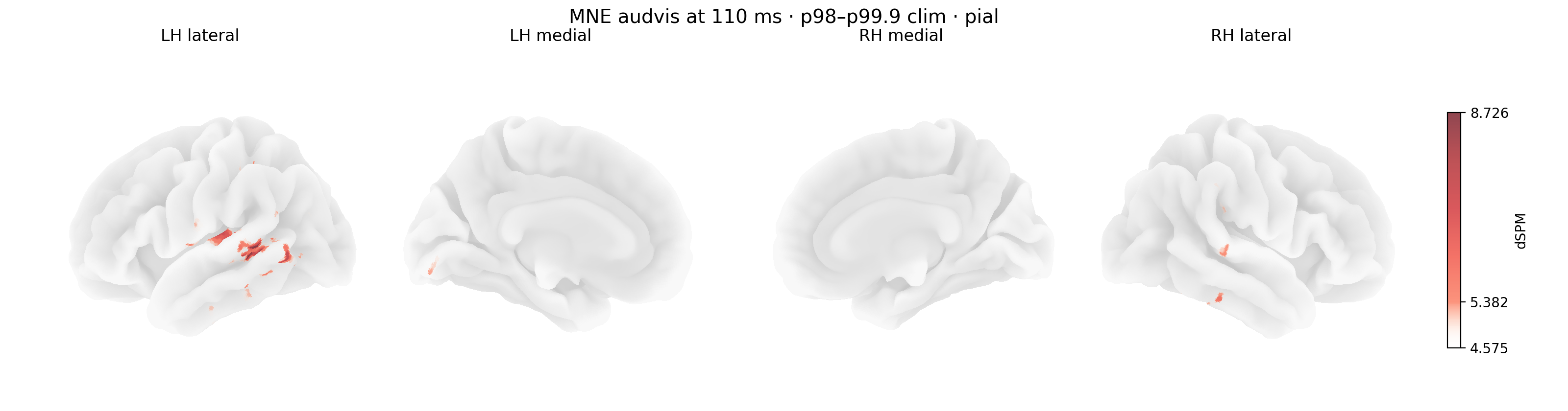
These pial views are included as optional anatomical presentations. They are not the recommended default for source-localization overviews. Use them when the relationship to native gyral and sulcal folding is itself important. Both images use the same pial geometry, source estimate, selected 110 ms sample, interpolation, threshold, and p98-p99.9 color controls; only the final renderer changes.

Installation

PySourceviz supports Python 3.9 or newer. A virtual environment is recommended. Install the package from PyPI with its default BrainSpace renderer:

python -m pip install PySourceviz

To use the optional Nilearn renderer as well, install the nilearn extra:

python -m pip install "PySourceviz[nilearn]"

Upgrade an existing installation to the latest PyPI release:

python -m pip install --upgrade PySourceviz

To reproduce results with this documented release, install version 0.1.0 explicitly:

python -m pip install "PySourceviz==0.1.0"

Verify the installed version:

python -c "import pysourceviz; print(pysourceviz.__version__)"

Quickstart

Load an MNE surface STC, point subjects_dir to the directory that contains the matching FreeSurfer subject, and save a PNG:

from pathlib import Path

import mne

from pysourceviz import plot_source


stc = mne.read_source_estimate("/data/inverse/audvis")
subjects_dir = Path("/data/freesurfer/subjects")

info = plot_source(
    stc,
    subjects_dir=subjects_dir,
    backend="brainspace",
    template="native",
    time=0.112,
    units="dSPM",
    title="Auditory response · 112 ms request",
    output="figures/audvis_112ms.png",
)

print(info["selected_time"])  # actual nearest STC sample, for example 0.11
print(info["color_range"])    # shared whole-brain display range
print(info["output"])         # resolved PNG path

Render the same prepared source map with Nilearn by changing one argument:

nilearn_info = plot_source(
    stc,
    subjects_dir=subjects_dir,
    backend="nilearn",
    template="native",
    time=0.112,
    clim={"kind": "percent", "lims": [98, 99, 99.9]},
    units="dSPM",
    title="Auditory response · Nilearn",
    output="figures/audvis_112ms_nilearn.png",
)

Time selection, interpolation, threshold, clim, colormap, layout, output size, and returned scientific metadata have the same meaning for both backends. Nilearn is imported only when backend="nilearn" is selected.

For stc.subject == "fsaverage", the example expects files such as /data/freesurfer/subjects/fsaverage/surf/lh.inflated. subjects_dir is one level above the subject; it is not the fsaverage directory itself.

Complete usage reference

The recipes below enumerate every supported source family and public control. All time values are seconds. PySourceviz never modifies the input STC.

Supported source-estimate families

MNE object	PySourceviz v0.1 behavior
mne.SourceEstimate	Real scalar cortical data; supports mode="magnitude" and mode="signed".
mne.VectorSourceEstimate	Cortical vector magnitude; signed display is not defined.
mne.MixedSourceEstimate	Uses only the cortical surface component.
mne.MixedVectorSourceEstimate	Uses the cortical surface component and converts vectors to magnitude.
mne.VolSourceEstimate / mne.VolVectorSourceEstimate	Unsupported volume-only data; use a volume plotting workflow instead.

Complex STCs are unsupported. PySourceviz also does not compute inverse solutions or silently turn volumetric results into cortical surface data.

Choose BrainSpace or Nilearn

BrainSpace is the backward-compatible default and uses VTK. Nilearn is an optional Matplotlib-based renderer:

plot_source(
    stc,
    subjects_dir=subjects_dir,
    backend="brainspace",
    time=0.112,
    output="brainspace.png",
)

plot_source(
    stc,
    subjects_dir=subjects_dir,
    backend="nilearn",
    time=0.112,
    output="nilearn.png",
)

Both calls pass the same prepared vertex arrays to the selected renderer. A static-only save returns info["plotter"] is None. Without a static-only save, that field contains a BrainSpace plotter or a Matplotlib Figure, respectively. Call .close() on a retained BrainSpace plotter or matplotlib.pyplot.close(info["plotter"]) on a retained Nilearn figure when it is no longer needed.

Select a time or reduce a time window

time=None is valid for an STC that already has exactly one sample:

plot_source(single_time_stc, subjects_dir=subjects_dir, time=None)

A numeric request chooses the nearest actual sample. time="peak" chooses the sample containing the largest whole-brain magnitude:

plot_source(stc, subjects_dir=subjects_dir, time=0.112)
plot_source(stc, subjects_dir=subjects_dir, time="peak")

For an inclusive window, use either the signed/absolute mean or non-negative RMS reduction:

plot_source(
    stc,
    subjects_dir=subjects_dir,
    time_window=(0.080, 0.160),
    reduce="mean",
)

plot_source(
    stc,
    subjects_dir=subjects_dir,
    time_window=(0.080, 0.160),
    reduce="rms",
    mode="magnitude",
)

time and time_window are mutually exclusive. Signed RMS is rejected because RMS has no sign.

Choose native, fsaverage, or another matching subject

template="native" resolves to stc.subject. An explicit subject name must match stc.subject:

plot_source(
    stc_native,
    subjects_dir=subjects_dir,
    template="native",
    time=0.112,
)

plot_source(
    stc_fsaverage,
    subjects_dir=subjects_dir,
    template="fsaverage",
    time=0.112,
)

plot_source(
    stc_study_average,
    subjects_dir=subjects_dir,
    template="my_study_average",
    time=0.112,
)

Cross-subject registration is deliberately external. Morph first with MNE, then plot the already matching result:

import mne


morph = mne.compute_source_morph(
    stc_native,
    subject_from=stc_native.subject,
    subject_to="fsaverage",
    subjects_dir=subjects_dir,
)
stc_fsaverage = morph.apply(stc_native)

plot_source(
    stc_fsaverage,
    subjects_dir=subjects_dir,
    template="fsaverage",
    time=0.112,
    output="subject_on_fsaverage.png",
)

Choose cortical anatomy and display interpolation

All three supported FreeSurfer surfaces are explicit:

plot_source(stc, subjects_dir=subjects_dir, time=0.112, surface="inflated")
plot_source(stc, subjects_dir=subjects_dir, time=0.112, surface="pial")
plot_source(stc, subjects_dir=subjects_dir, time=0.112, surface="white")

inflated is the recommended default for source-localization overview figures. It unfolds buried cortex without changing the data assigned to each vertex. Use pial when the relationship to native cortical folding is itself important, and white when the gray-white boundary is the intended anatomy; neither alternative changes the inverse solution.

Sparse source vertices can be expanded to the display mesh in three ways:

# Recommended default: let MNE propagate until the surface is covered.
plot_source(stc, subjects_dir=subjects_dir, time=0.112, smoothing_steps=None)

# Legacy piecewise-constant nearest-source assignment.
plot_source(
    stc,
    subjects_dir=subjects_dir,
    time=0.112,
    smoothing_steps="nearest",
)

# Exact non-negative number of adjacency-propagation iterations.
plot_source(stc, subjects_dir=subjects_dir, time=0.112, smoothing_steps=5)

This is same-subject display interpolation, not Gaussian or statistical smoothing. Thresholds and color limits are computed from original sparse values before display expansion.

Choose magnitude or signed color semantics

Magnitude is non-negative and defaults to the sequential Reds colormap:

plot_source(
    stc,
    subjects_dir=subjects_dir,
    time=0.112,
    mode="magnitude",
    cmap="Reds",
    units="dSPM",
)

Signed scalar data default to RdBu_r and a symmetric range:

plot_source(
    stc_scalar,
    subjects_dir=subjects_dir,
    time_window=(0.080, 0.160),
    reduce="mean",
    mode="signed",
    output="signed_mean.png",
)

Signed mode is unavailable for vector and mixed-vector STCs.

Choose a threshold and color limits

Leave the hard display mask disabled, use a numerical cutoff, or resolve a percentile from the combined sparse hemispheres:

plot_source(stc, subjects_dir=subjects_dir, time=0.112, threshold=None)
plot_source(stc, subjects_dir=subjects_dir, time=0.112, threshold=3.0)
plot_source(stc, subjects_dir=subjects_dir, time=0.112, threshold="95%")

Color limits support a robust percentile, an explicit range, and MNE-style three-control dictionaries:

plot_source(stc, subjects_dir=subjects_dir, time=0.112, clim="robust")

plot_source(stc, subjects_dir=subjects_dir, time=0.112, clim=(0.0, 12.5))

plot_source(
    stc,
    subjects_dir=subjects_dir,
    time=0.112,
    clim={"kind": "percent", "lims": [98, 99, 99.9]},
)

plot_source(
    stc,
    subjects_dir=subjects_dir,
    time=0.112,
    clim={"kind": "value", "lims": [3.0, 4.0, 6.0]},
)

plot_source(
    stc_signed,
    subjects_dir=subjects_dir,
    time=0.112,
    mode="signed",
    clim={"kind": "percent", "pos_lims": [95, 99, 99.9]},
)

robust_percentile=98.0 changes the percentile used by clim="robust". For dictionary clim, the lower, middle, and upper controls set the start of the visibility ramp, the middle palette color/full overlay opacity, and the saturation point. These controls and thresholds are visualization choices, not tests of statistical significance.

Choose layout, styling, and output behavior

Use a four-panel row or a two-by-two grid, and optionally control the rest of the presentation:

plot_source(stc, subjects_dir=subjects_dir, time=0.112, layout="row")
plot_source(stc, subjects_dir=subjects_dir, time=0.112, layout="grid")

plot_source(
    stc,
    subjects_dir=subjects_dir,
    time=0.112,
    title="Auditory response",
    colorbar=False,
    background="white",
    size=(1600, 420),
    scale=(2, 2),
    output="auditory.png",
)

plot_source(
    stc,
    subjects_dir=subjects_dir,
    time=0.112,
    background=(1.0, 1.0, 1.0),
    transparent=True,
    output="auditory_transparent.png",
)

The output/display combinations are:

# Save a PNG and close the static renderer (show defaults to False here).
saved = plot_source(
    stc,
    subjects_dir=subjects_dir,
    time=0.112,
    output="source.png",
)

# Open an interactive window (show defaults to True with no output).
interactive = plot_source(stc, subjects_dir=subjects_dir, time=0.112, show=True)

# Save and also create a separate interactive scene.
both = plot_source(
    stc,
    subjects_dir=subjects_dir,
    time=0.112,
    output="source_and_window.png",
    show=True,
)

# Retain an offscreen plotter without saving or opening a window.
offscreen = plot_source(stc, subjects_dir=subjects_dir, time=0.112, show=False)
offscreen["plotter"].close()

output accepts PNG paths only and creates missing parent directories. The default logical size is 1600 x 420 for layout="row" and 900 x 760 for layout="grid"; screenshot scale=(2, 2) doubles both pixel axes.

Compare conditions with one shared scale

Use the same preregistered or pooled range for every condition instead of a separate robust range per image:

shared_clim = (0.0, 12.5)

info_a = plot_source(
    stc_condition_a,
    subjects_dir=subjects_dir,
    time=0.112,
    clim=shared_clim,
    title="Condition A",
    output="condition_a.png",
)
info_b = plot_source(
    stc_condition_b,
    subjects_dir=subjects_dir,
    time=0.112,
    clim=(0.0, 12.5),
    title="Condition B",
    output="condition_b.png",
)

assert info_a["color_range"] == info_b["color_range"] == shared_clim

Inspect returned metadata

Every call returns a dictionary containing the resolved template and surface, interpolation setting, time/window selection, threshold, whole-brain color range and control points, colormap, layout, logical/pixel size controls, output path, and plotter. Useful checks include:

for key in (
    "backend",
    "template",
    "surface",
    "smoothing_steps",
    "selected_time",
    "sampled_time_window",
    "threshold",
    "color_range",
    "color_control_points",
    "output",
):
    print(key, info[key])

Run the bundled examples

Program	Purpose
examples/basic_usage.py	Reusable BrainSpace/Nilearn fixed-time, window-RMS, and shared-clim helpers.
examples/real_data_validation.py	Five-image acceptance set plus a JSON provenance manifest.
examples/compare_nilearn_backend.py	Controlled BrainSpace/Nilearn comparison from one surface STC.

python examples/basic_usage.py

python examples/real_data_validation.py \
    --stc-base /data/fsaverage_audvis_trunc-meg \
    --subjects-dir /data/subjects \
    --subject fsaverage \
    --output-dir validation-output

python examples/compare_nilearn_backend.py \
    --stc-base /data/fsaverage_audvis_trunc-meg \
    --subjects-dir /data/subjects \
    --subject fsaverage \
    --output-dir renderer-comparison

Complete plot_source() parameter reference

The table is synchronized with the public function signature. “Required” means there is no default; all arguments after stc are keyword-only.

Parameter	Default	Accepted values and effect
stc	required	Real mne.SourceEstimate, vector surface STC, or mixed STC with a cortical component.
subjects_dir	required	Path containing the matching FreeSurfer subject directory.
backend	"brainspace"	"brainspace" or optional "nilearn"; scientific preprocessing is shared.
template	"native"	"native" or an explicit subject name equal to stc.subject.
surface	"inflated"	"inflated", "pial", or "white".
smoothing_steps	None	Automatic MNE coverage, "nearest", or a non-negative integer.
time	None	Seconds, "peak", or None; mutually exclusive with time_window.
time_window	None	Inclusive (start, stop) seconds or None.
reduce	"mean"	"mean" or "rms" for a time window.
mode	"magnitude"	"magnitude" or scalar "signed".
threshold	None	Non-negative number, percentile string such as "95%", or None.
clim	"robust"	"robust", (lower, upper), or MNE-style three-control dictionary.
robust_percentile	98.0	Percentile in (0, 100] used by robust limits.
cmap	None	Matplotlib colormap name or mode-aware default.
units	None	Optional activation colorbar title.
layout	"row"	"row" or "grid".
title	None	Optional figure title.
colorbar	True	Show or hide the shared activation colorbar.
background	"white"	Matplotlib color name or RGB triple.
output	None	Optional .png path; missing parent directories are created.
size	None	Logical (width, height) or the layout-specific default.
scale	(2, 2)	Positive integer screenshot scale for each pixel axis.
transparent	False	Use an alpha background for saved PNG output.
show	None	True, False, or output-aware default behavior.

FreeSurfer subjects_dir in detail

For subject="sample" and surface="inflated", PySourceviz reads:

<subjects_dir>/sample/surf/lh.inflated
<subjects_dir>/sample/surf/rh.inflated
<subjects_dir>/sample/surf/lh.sulc
<subjects_dir>/sample/surf/rh.sulc
<subjects_dir>/sample/label/lh.cortex.label
<subjects_dir>/sample/label/rh.cortex.label

Missing surface or sulc files are fatal and their full paths appear in the error. Missing cortex labels emit one warning and disable medial wall masking for the affected hemisphere, so install or generate those labels before making final figures.

Display interpolation and source-space resolution

smoothing_steps=None asks MNE to propagate sparse source values over surface adjacency until the display mesh is covered. smoothing_steps="nearest" reproduces the piecewise-constant legacy view. A non-negative integer requests an exact number of propagation iterations; if it is too small for a dense mesh, MNE warns rather than pretending the surface was completely filled.

Interpolation is applied to a one-time display copy. Numeric/percentile thresholds, robust limits, and percent clim controls are computed from combined left/right sparse values before expansion, so repeated dense vertices cannot bias a percentile. The input STC is unchanged.

Very coarse inverse source spaces can remain visibly patchy even with automatic interpolation. For scientifically smoother spatial detail, improve the source-space resolution in the forward/inverse model or use an explicitly reported analysis-stage smoothing method. Do not hide a low-resolution inverse solution with undocumented plotting-only Gaussian blur.

Display threshold, color limits, and inference

A threshold is an optional hard display mask: values below it become fully transparent after surface expansion. Abrupt masking can make isolated patches look prominent. MNE-style clim dictionaries instead create a gradual transparent-to-visible transition around peak regions.

The bundled audvis reference uses:

clim={"kind": "percent", "lims": [98, 99, 99.9]}

It starts the ramp at the 98th percentile, reveals more localized activation than the stricter p99 example, and avoids a cortex-wide red cast. Signed data use pos_lims with a diverging palette.

Neither threshold nor clim performs a statistical significance test, multiple-comparison correction, or inference. Determine significance in the analysis pipeline, then choose display controls that faithfully communicate that result. When color must be quantitatively comparable, use a shared clim for every condition.

Layout, PNG output, and metadata

The row layout is LH lateral | LH medial | RH medial | RH lateral. The grid places LH/RH lateral views on the first row and LH/RH medial views on the second. BrainSpace uses global camera rotations internally; the anatomical labels describe the hemisphere-relative view shown to the reader.

Static-only output returns plotter=None. Interactive or explicitly retained scenes return a BrainSpace plotter or Nilearn Matplotlib Figure, according to backend. The caller should close retained renderer objects. Returned selected_time is always an actual STC sample, and sampled_time_window records the first and last samples included in a window.

Reproduce the real-data acceptance set

The workflow follows MNE's source-estimate visualization tutorial. With an existing MNE sample dataset:

python examples/real_data_validation.py \
    --sample-data-dir /path/to/MNE-sample-data \
    --output-dir validation-output

Or use an explicit two-hemisphere STC base and subject anatomy:

python examples/real_data_validation.py \
    --stc-base /data/fsaverage_audvis_trunc-meg \
    --subjects-dir /data/subjects \
    --subject fsaverage \
    --output-dir validation-output

The script creates fixed 112 ms, RMS 80-160 ms, inflated, pial, and shared-clim comparison images plus validation.json. Its 0.65x comparison control checks display consistency only; it is not an independent experimental condition. --download opts into MNE's roughly 1.45 GB sample download. The default never starts that download.

Compare the built-in BrainSpace and Nilearn renderers

Install the optional backend in an editable source checkout:

python -m pip install -e ".[nilearn]"

The repository keeps comparison as a compatibility alias for the controlled acceptance workflow:

python -m pip install -e ".[comparison]"

Nilearn's plot_img_on_surf accepts a 3D Niimg-like volume and projects voxels onto a surface. An MNE surface SourceEstimate already contains values at cortical vertices, so converting it to a volume and projecting it back would add interpolation and would not be a controlled renderer comparison. The PySourceviz Nilearn backend therefore keeps the shared time selection, display interpolation, medial-wall mask, threshold, colormap, and color range, then passes the same vertex arrays to Nilearn's plot_surf_stat_map.

The often-cited plot_img_on_surf gallery image is a different data case. Its 3D motor statistical map has negative and positive voxels, uses a diverging RdBu_r palette, and projects multiple volumetric samples near the cortical depth/normal. The audvis dSPM reference here is non-negative at the selected sample, so the sequential Reds palette is scientifically appropriate rather than inventing a blue negative branch.

Run the controlled comparison with explicit settings:

python examples/compare_nilearn_backend.py \
    --stc-base /data/fsaverage_audvis_trunc-meg \
    --subjects-dir /data/subjects \
    --subject fsaverage \
    --time 0.112 \
    --surface inflated \
    --smoothing-steps auto \
    --clim-percent 98 99 99.9 \
    --mode magnitude \
    --cmap Reds \
    --output-dir renderer-comparison

The comparison defaults to the recommended surface="inflated" and automatic interpolation (smoothing_steps=None; CLI spelling --smoothing-steps auto). It creates brainspace.png, nilearn.png, and comparison.json. Both images share the 1600 x 420 logical canvas, four-view order, source sample, activation array, sulcal anatomy, cmap, and (vmin, vmax). To inspect native folding explicitly, pass --surface pial; to inspect the gray-white boundary, pass --surface white.

The manifest records source/surface vertex counts, density ratio, versions, pixel sizes, display_value_range, and display_sign_counts. BrainSpace/VTK and Nilearn/Matplotlib can still look different because VTK shades point-data actors, while Nilearn uses mean vertex-to-face averaging on triangular faces. This affects surface appearance, not the prepared source values. Use plot_img_on_surf only when the source result genuinely is a 3D NIfTI volume and the volume-to-surface projection is scientifically intended.

Building and publishing

For an editable development environment with tests and release tools:

python -m pip install -e ".[dev]"
python -m pytest -q

The release helper resolves the project root from its own location. From the repository root, run:

./scripts/release.sh build
./scripts/release.sh testpypi --clean
# After installing and testing the TestPyPI candidate:
./scripts/release.sh pypi --reuse

Every target builds with PEP 517 unless --reuse is selected, and runs Twine's strict metadata check before any upload. --clean removes only old .tar.gz and .whl files. --reuse rechecks and uploads the exact existing pair, so the PyPI release can match the tested TestPyPI artifacts. Production upload asks for publish; use --yes only for an intentional non-interactive release. Override the interpreter or output directory with PYSOURCEVIZ_PYTHON or PYSOURCEVIZ_DIST_DIR. Without --clean or --reuse, the helper refuses to overwrite existing distributions. Run ./scripts/release.sh --help for the complete command reference.

For the equivalent manual workflow, update the version in pyproject.toml, make sure dist/ contains no artifacts from an older version, then build both the source distribution and wheel with the modern PEP 517 frontend:

The PyPI long description cannot resolve repository-relative images, so this README uses GitHub Raw URLs. Always push the release commit containing the gallery assets to GitHub before either upload so all five result images are already reachable.

python -m build
python -m twine check --strict dist/*

Upload to TestPyPI first and install the candidate without resolving runtime dependencies from the test index:

python -m twine upload --repository testpypi dist/*
python -m pip install --index-url https://test.pypi.org/simple/ --no-deps PySourceviz

After testing the candidate, publish the same checked artifacts to PyPI:

python -m twine upload dist/*

Enter an API token through Twine/keyring or the upload prompt; never write a token into this repository. See the official PyPA packaging tutorial for the standards-based build and upload flow.

Common errors

Message or symptom	Meaning and action
template='native' requires stc.subject	Set the STC subject when creating/loading it, or use a correctly matching explicit template.
STC subject space ... does not match	Morph the STC externally with mne.compute_source_morph; do not relabel it.
Required FreeSurfer surface file(s) missing	Point subjects_dir one level above the subject and install the requested surface plus lh/rh.sulc.
Cortex label file(s) missing warning	Medial wall masking is disabled for that hemisphere; restore lh/rh.cortex.label before final export.
STC has multiple time samples	Set time, time="peak", or time_window.
Large piecewise-constant activation patches	Use smoothing_steps=None; if a coarse source-space resolution remains visible, improve the inverse model instead of adding hidden plotting blur.
output must use the .png extension	Export PNG directly; convert formats afterward if needed.
backend="nilearn" requires the optional Nilearn renderer	Install PySourceviz[nilearn], then rerun the same call.
Native VTK window/backend failure	Configure a supported VTK backend for the machine or render in a desktop session.

Known limits

PySourceviz v0.1 renders real cortical scalar STCs, vector-surface magnitude, and the surface portion of mixed STCs through BrainSpace or optional Nilearn. It does not render volume-only or complex STCs, compute inverse solutions, perform cross-subject morphing, or conduct statistical inference. Its same-subject adjacency propagation is display interpolation; it must not be interpreted as Gaussian/statistical smoothing or an increase in source-space resolution.